In [1]:
%%HTML
<link rel="stylesheet" type="text/css" href="https://raw.githubusercontent.com/malkaguillot/Foundations-in-Data-Science-and-Machine-Learning/refs/heads/main/docs/utils/custom.css">
%%HTML
<link rel="stylesheet" type="text/css" href="../utils/custom.css">
%%HTML
What is (modern) pandas?
In [2]:
import pandas as pd
What is pandas?
- Industry standard DataFrame library in Python
- Covers all you need for data management
- Loading datasets in many formats
- Cleaning data
- Generating variables
- Reshaping datasets
- Compatible with all plotting and statistics libraries
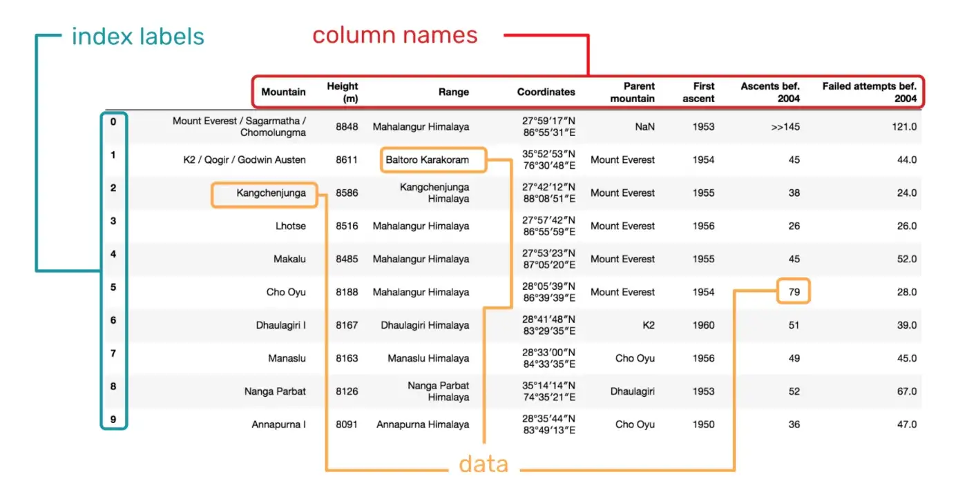
What is a DataFrame?
- Tabular data format, typically loaded from a file
- Two mental models:
- Matrix/Array with labels
- Dictionary of columns
- Variables are columns
- Observations are rows
- Can be manipulated in Python
DataFrame and Series
Creating a DataFrame
- Data for a DataFrame can be nested lists or similar things
- Columns and index can be ints, strings and tuples
- Powerful strategy: Whenever you learn pandas or debug problems, create tiny DataFrames and Series to gain better understanding
In [3]:
df = pd.DataFrame(
data=[[1, "bla"], [3, "blubb"]],
columns=["a", "b"],
index=["c", "d"]
)
df
Out[3]:
| a | b | |
|---|---|---|
| c | 1 | bla |
| d | 3 | blubb |
Creating a DataFrame from a dictionary
In [4]:
df = pd.DataFrame(
data={
"a": [1, 3],
"b": ["bla", "blubb"]
},
index=["c", "d"]
)
df
Out[4]:
| a | b | |
|---|---|---|
| c | 1 | bla |
| d | 3 | blubb |
What is a Series?
- Each column of a DataFrame is a Series
- Mental model: Vector with an index
- All entries in a Series have the same dtype
Creating a Series
In [5]:
pd.Series(
[3.0, 4.5], index=["x", "y"],
)
Out[5]:
x 3.0 y 4.5 dtype: float64
Assignment is index aligned!
- New columns can be assigned with square brackets
- Index is automatically aligned!
- Makes many things safer!
- Can make pandas slow
In [6]:
sr = pd.Series(
[3.0, 4.5], index=["c", "d"],
)
df["new_col"] = sr
df
Out[6]:
| a | b | new_col | |
|---|---|---|---|
| c | 1 | bla | 3.0 |
| d | 3 | blubb | 4.5 |
Data types
The need for different data types
- Each column has a dtype
- Enables efficient storage and fast computation
- Dtypes are not always set optimally after loading data
In [8]:
df.dtypes
Out[8]:
Unnamed: 0 int64 serial int64 country object description object designation object points int64 price float64 province object region_1 object region_2 object taster_name object taster_twitter_handle object title object variety object winery object dtype: object
Benefits of good type representation
- Fast calculations in a low level language
- Access to operations that are only relevant for some types
- Memory efficiency
Converting to efficient dtypes
In [9]:
better_dtypes = {
"country": pd.CategoricalDtype(),
"points": pd.UInt8Dtype(),
"price": pd.Float32Dtype(),
}
df = df.astype(better_dtypes)
df.dtypes
Out[9]:
Unnamed: 0 int64 serial int64 country category description object designation object points UInt8 price Float32 province object region_1 object region_2 object taster_name object taster_twitter_handle object title object variety object winery object dtype: object
Overview of numeric dtypes
| Type | Properties |
|---|---|
| pd.Int8Dtype() | Byte (-128 to 127) |
| pd.Int16Dtype() | Integer (-32768 to 32767) |
| pd.Int32Dtype() | Integer (-2147483648 to 2147483647) |
| pd.Int64Dtype() | Integer (-9223372036854775808 to 9223372036854775807) |
| pd.UInt8Dtype() | Unsigned Integer (0 to 255) |
| pd.UInt16Dtype() | Unsigned Integer (0 to 65535) |
| pd.UInt32Dtype() | Unsigned Integer (0 to 4294967295) |
| pd.UInt64Dtype() | Unsigned Integer (0 to 18446744073709551615) |
| pd.Float32Dtype() | Float (3.4028235e+38 to 1.4012985e-45) |
| pd.Float64Dtype() | Float (double precision float) |
String vs. Categorical
pd.CategoricalDtype()is for data that takes on a limited number of values- Internally stored as integers
- Vert fast relabeling or resorting of categories
pd.StringDtype()is for actual text data- Internally stored as
pyarrowarray - Fast string functions similar to
strin Python
- Internally stored as
Working with Strings
- The
.straccessor provides access to the string methods - Vectorized and fast implementations!
In [10]:
sr = pd.Series(["Guido", "Tim", "Raymond"])
sr.str.lower()
Out[10]:
0 guido 1 tim 2 raymond dtype: object
In [11]:
sr.str.replace("i", "iii")
Out[11]:
0 Guiiido 1 Tiiim 2 Raymond dtype: object
Other examples:
src.str.lensrc.str.contains
See this tutorial for more string methods
Working with categoricals
- Categories are defined independent of data
- Protection against invalid categories
- Good for visualization!
sr.cataccessor provides access to methods- See this tutorial for more method
In [12]:
cat_type = pd.CategoricalDtype(
categories=["low", "middle", "high"],
ordered=True,
)
sr = pd.Series(
["low", "high", "high"],
dtype=cat_type,
)
sr
Out[12]:
0 low 1 high 2 high dtype: category Categories (3, object): ['low' < 'middle' < 'high']
Loading and saving data

Example: Loading a csv file
- first argument is the file name (with relative or absolute path)
engine="pyarrow"ensures we are getting modern pandas dtypes- many other optional arguments
In [13]:
df = pd.read_csv(
"https://raw.githubusercontent.com/HSG-8276-Spring-2025/class-ressources/refs/heads/main/data/winemag-data-130k-v3.csv", index_col=0,
engine="pyarrow"
)
df.head()
Out[13]:
| Unnamed: 0 | serial | country | description | designation | points | price | province | region_1 | region_2 | taster_name | taster_twitter_handle | title | variety | winery | |
|---|---|---|---|---|---|---|---|---|---|---|---|---|---|---|---|
| 0 | 0 | 0 | Italy | Aromas include tropical fruit, broom, brimston... | Vulkà Bianco | 87 | NaN | Sicily & Sardinia | Etna | None | Kerin O’Keefe | @kerinokeefe | Nicosia 2013 Vulkà Bianco (Etna) | White Blend | Nicosia |
| 1 | 1 | 1 | Portugal | This is ripe and fruity, a wine that is smooth... | Avidagos | 87 | 15.0 | Douro | None | None | Roger Voss | @vossroger | Quinta dos Avidagos 2011 Avidagos Red (Douro) | Portuguese Red | Quinta dos Avidagos |
| 2 | 2 | 2 | US | Tart and snappy, the flavors of lime flesh and... | None | 87 | 14.0 | Oregon | Willamette Valley | Willamette Valley | Paul Gregutt | @paulgwine | Rainstorm 2013 Pinot Gris (Willamette Valley) | Pinot Gris | Rainstorm |
| 3 | 3 | 3 | US | Pineapple rind, lemon pith and orange blossom ... | Reserve Late Harvest | 87 | 13.0 | Michigan | Lake Michigan Shore | None | Alexander Peartree | None | St. Julian 2013 Reserve Late Harvest Riesling ... | Riesling | St. Julian |
| 4 | 4 | 4 | US | Much like the regular bottling from 2012, this... | Vintner's Reserve Wild Child Block | 87 | 65.0 | Oregon | Willamette Valley | Willamette Valley | Paul Gregutt | @paulgwine | Sweet Cheeks 2012 Vintner's Reserve Wild Child... | Pinot Noir | Sweet Cheeks |
Other read functions
| Reader | Extension | Comment |
|---|---|---|
| pd.read_csv | .csv | Often need to use optional arguments to make it work |
| pd.read_pickle | .pkl | Good for intermediate files; Python specific. |
| pd.read_feather | .arrow | Very modern and powerful file format. |
| pd.read_stata | .dta | Stata’s proprietary format. Avoid if you can. |
File format recommendations
- Use
.pklformat for processed datasets that you do not share with others- Very fast to read and write
- Preserves every aspect of your DataFrame (e.g. dtypes)
- Use
.parquetto save files you want to share with others- Can be read by many languages and programs
- Efficient compression
- Use
.dtaiff sharing with Stata users
Setting and renaming columns and indices
Why the Index is important
- We have seen that pandas aligns new columns in a DataFrame by index
- Many other operations are aligned by index
- Using a meaningful index makes this even safer
- Index should be unique and not contain floats
Setting and resetting the index
set_indexandreset_indexare inverse functionsset_indexcan take any column or list of columns- Optional argument
drop=Trueordrop=Falsedetermines what happens with the old index inset_index
In [14]:
df.index
Out[14]:
Index([ 0, 1, 2, 3, 4, 5, 6, 7, 8,
9,
...
129961, 129962, 129963, 129964, 129965, 129966, 129967, 129968, 129969,
129970],
dtype='int64', name='', length=129971)
In [15]:
df = df.set_index(["country", "winery"])
df.index
Out[15]:
MultiIndex([( 'Italy', 'Nicosia'),
('Portugal', 'Quinta dos Avidagos'),
( 'US', 'Rainstorm'),
( 'US', 'St. Julian'),
( 'US', 'Sweet Cheeks'),
( 'Spain', 'Tandem'),
( 'Italy', 'Terre di Giurfo'),
( 'France', 'Trimbach'),
( 'Germany', 'Heinz Eifel'),
( 'France', 'Jean-Baptiste Adam'),
...
( 'Italy', 'COS'),
( 'Italy', 'Cusumano'),
( 'Israel', 'Dalton'),
( 'France', 'Domaine Ehrhart'),
( 'France', 'Domaine Rieflé-Landmann'),
( 'Germany', 'Dr. H. Thanisch (Erben Müller-Burggraef)'),
( 'US', 'Citation'),
( 'France', 'Domaine Gresser'),
( 'France', 'Domaine Marcel Deiss'),
( 'France', 'Domaine Schoffit')],
names=['country', 'winery'], length=129971)
In [16]:
df = df.reset_index()
df.index
Out[16]:
RangeIndex(start=0, stop=129971, step=1)
Renaming columns
- Dict can contain only the subset of variables that is actually renamed
- Renaming the index works the same way but is rarely needed
In [17]:
df.columns
Out[17]:
Index(['country', 'winery', 'Unnamed: 0', 'serial', 'description',
'designation', 'points', 'price', 'province', 'region_1', 'region_2',
'taster_name', 'taster_twitter_handle', 'title', 'variety'],
dtype='object')
In [18]:
new_names = {
"country": "country name",
"taster_name": "taster name",
}
df = df.rename(columns=new_names)
df.columns
Out[18]:
Index(['country name', 'winery', 'Unnamed: 0', 'serial', 'description',
'designation', 'points', 'price', 'province', 'region_1', 'region_2',
'taster name', 'taster_twitter_handle', 'title', 'variety'],
dtype='object')
- Instead of a dict, you can provide a function that converts old names to new names!
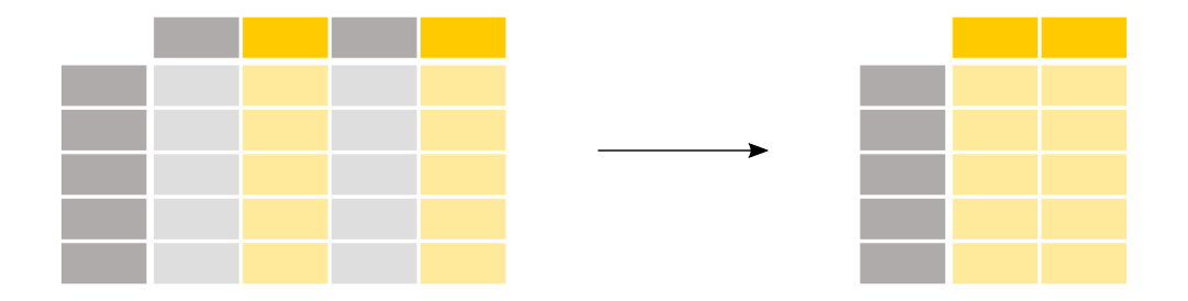
Selecting rows and columns
In [19]:
df['country name'].head(6)
Out[19]:
0 Italy 1 Portugal 2 US 3 US 4 US 5 Spain Name: country name, dtype: object
- For multiple columns you need double brackets:
- Outer: selecting columns
- Inner: defining a list of variables
In [20]:
df[['country name', 'taster name']]
Out[20]:
| country name | taster name | |
|---|---|---|
| 0 | Italy | Kerin O’Keefe |
| 1 | Portugal | Roger Voss |
| 2 | US | Paul Gregutt |
| 3 | US | Alexander Peartree |
| 4 | US | Paul Gregutt |
| ... | ... | ... |
| 129966 | Germany | Anna Lee C. Iijima |
| 129967 | US | Paul Gregutt |
| 129968 | France | Roger Voss |
| 129969 | France | Roger Voss |
| 129970 | France | Roger Voss |
129971 rows × 2 columns

In [21]:
df.loc[1]
Out[21]:
country name Portugal winery Quinta dos Avidagos Unnamed: 0 1 serial 1 description This is ripe and fruity, a wine that is smooth... designation Avidagos points 87 price 15.0 province Douro region_1 None region_2 None taster name Roger Voss taster_twitter_handle @vossroger title Quinta dos Avidagos 2011 Avidagos Red (Douro) variety Portuguese Red Name: 1, dtype: object
- For a MultiIndex you can specify some or all levels
In [22]:
df = df.set_index(["country name", "winery"])
df.loc["Italy"]
Out[22]:
| Unnamed: 0 | serial | description | designation | points | price | province | region_1 | region_2 | taster name | taster_twitter_handle | title | variety | |
|---|---|---|---|---|---|---|---|---|---|---|---|---|---|
| winery | |||||||||||||
| Nicosia | 0 | 0 | Aromas include tropical fruit, broom, brimston... | Vulkà Bianco | 87 | NaN | Sicily & Sardinia | Etna | None | Kerin O’Keefe | @kerinokeefe | Nicosia 2013 Vulkà Bianco (Etna) | White Blend |
| Terre di Giurfo | 6 | 6 | Here's a bright, informal red that opens with ... | Belsito | 87 | 16.0 | Sicily & Sardinia | Vittoria | None | Kerin O’Keefe | @kerinokeefe | Terre di Giurfo 2013 Belsito Frappato (Vittoria) | Frappato |
| Masseria Setteporte | 13 | 13 | This is dominated by oak and oak-driven aromas... | Rosso | 87 | NaN | Sicily & Sardinia | Etna | None | Kerin O’Keefe | @kerinokeefe | Masseria Setteporte 2012 Rosso (Etna) | Nerello Mascalese |
| Baglio di Pianetto | 22 | 22 | Delicate aromas recall white flower and citrus... | Ficiligno | 87 | 19.0 | Sicily & Sardinia | Sicilia | None | Kerin O’Keefe | @kerinokeefe | Baglio di Pianetto 2007 Ficiligno White (Sicilia) | White Blend |
| Canicattì | 24 | 24 | Aromas of prune, blackcurrant, toast and oak c... | Aynat | 87 | 35.0 | Sicily & Sardinia | Sicilia | None | Kerin O’Keefe | @kerinokeefe | Canicattì 2009 Aynat Nero d'Avola (Sicilia) | Nero d'Avola |
| ... | ... | ... | ... | ... | ... | ... | ... | ... | ... | ... | ... | ... | ... |
| Col Vetoraz Spumanti | 129929 | 129929 | This luminous sparkler has a sweet, fruit-forw... | None | 91 | 38.0 | Veneto | Prosecco Superiore di Cartizze | None | None | None | Col Vetoraz Spumanti NV Prosecco Superiore di... | Prosecco |
| Baglio del Cristo di Campobello | 129943 | 129943 | A blend of Nero d'Avola and Syrah, this convey... | Adènzia | 90 | 29.0 | Sicily & Sardinia | Sicilia | None | Kerin O’Keefe | @kerinokeefe | Baglio del Cristo di Campobello 2012 Adènzia R... | Red Blend |
| Feudo Principi di Butera | 129947 | 129947 | A blend of 65% Cabernet Sauvignon, 30% Merlot ... | Symposio | 90 | 20.0 | Sicily & Sardinia | Terre Siciliane | None | Kerin O’Keefe | @kerinokeefe | Feudo Principi di Butera 2012 Symposio Red (Te... | Red Blend |
| COS | 129961 | 129961 | Intense aromas of wild cherry, baking spice, t... | None | 90 | 30.0 | Sicily & Sardinia | Sicilia | None | Kerin O’Keefe | @kerinokeefe | COS 2013 Frappato (Sicilia) | Frappato |
| Cusumano | 129962 | 129962 | Blackberry, cassis, grilled herb and toasted a... | Sàgana Tenuta San Giacomo | 90 | 40.0 | Sicily & Sardinia | Sicilia | None | Kerin O’Keefe | @kerinokeefe | Cusumano 2012 Sàgana Tenuta San Giacomo Nero d... | Nero d'Avola |
19540 rows × 13 columns
Selecting rows and columns
- Use
.loc[rows, columns]to select rows and columns - Can use everything seen before
In [23]:
df.loc["Italy", "taster name"]
/var/folders/cg/tgk7cwd906x_71j8jdd3gzc00000gn/T/ipykernel_90395/898296892.py:1: PerformanceWarning: indexing past lexsort depth may impact performance. df.loc["Italy", "taster name"]
Out[23]:
winery
Nicosia Kerin O’Keefe
Terre di Giurfo Kerin O’Keefe
Masseria Setteporte Kerin O’Keefe
Baglio di Pianetto Kerin O’Keefe
Canicattì Kerin O’Keefe
...
Col Vetoraz Spumanti None
Baglio del Cristo di Campobello Kerin O’Keefe
Feudo Principi di Butera Kerin O’Keefe
COS Kerin O’Keefe
Cusumano Kerin O’Keefe
Name: taster name, Length: 19540, dtype: object
In [24]:
df.loc[["Italy", "Australia"], ["taster name", "points"]]
Out[24]:
| taster name | points | ||
|---|---|---|---|
| country name | winery | ||
| Italy | Nicosia | Kerin O’Keefe | 87 |
| Terre di Giurfo | Kerin O’Keefe | 87 | |
| Masseria Setteporte | Kerin O’Keefe | 87 | |
| Baglio di Pianetto | Kerin O’Keefe | 87 | |
| Canicattì | Kerin O’Keefe | 87 | |
| ... | ... | ... | ... |
| Australia | Kilikanoon | None | 89 |
| Atze's Corner | None | 89 | |
| Moorooroo | None | 87 | |
| Mr. Riggs | None | 87 | |
| Henschke | Joe Czerwinski | 90 |
21869 rows × 2 columns
In [25]:
df = df.reset_index()
Selecting rows using Boolean Series
- Comparisons of Series produceBoolean Series!
- Complex conditions with
|and& - Boolean Series can be used for selecting rows
- Works also inside
.loc
In [26]:
df['points']>88
Out[26]:
0 False
1 False
2 False
3 False
4 False
...
129966 True
129967 True
129968 True
129969 True
129970 True
Name: points, Length: 129971, dtype: bool
In [27]:
df = df[['country name', 'points', 'price', "taster name"]]
Using the Booleans Series
In [28]:
df[df['points']>88]
Out[28]:
| country name | points | price | taster name | |
|---|---|---|---|---|
| 119 | France | 92 | 80.0 | None |
| 120 | Italy | 92 | 70.0 | None |
| 121 | US | 92 | 36.0 | None |
| 122 | US | 92 | 39.0 | None |
| 123 | Australia | 92 | 40.0 | Joe Czerwinski |
| ... | ... | ... | ... | ... |
| 129966 | Germany | 90 | 28.0 | Anna Lee C. Iijima |
| 129967 | US | 90 | 75.0 | Paul Gregutt |
| 129968 | France | 90 | 30.0 | Roger Voss |
| 129969 | France | 90 | 32.0 | Roger Voss |
| 129970 | France | 90 | 21.0 | Roger Voss |
61271 rows × 4 columns
Inspecting and summarizing data
- Real datasets don’t fit on a screen
- Need quick ways to:
- Look at subsets
- Calculate summary statistics
- Plot distributions
In [29]:
df
Out[29]:
| country name | points | price | taster name | |
|---|---|---|---|---|
| 0 | Italy | 87 | NaN | Kerin O’Keefe |
| 1 | Portugal | 87 | 15.0 | Roger Voss |
| 2 | US | 87 | 14.0 | Paul Gregutt |
| 3 | US | 87 | 13.0 | Alexander Peartree |
| 4 | US | 87 | 65.0 | Paul Gregutt |
| ... | ... | ... | ... | ... |
| 129966 | Germany | 90 | 28.0 | Anna Lee C. Iijima |
| 129967 | US | 90 | 75.0 | Paul Gregutt |
| 129968 | France | 90 | 30.0 | Roger Voss |
| 129969 | France | 90 | 32.0 | Roger Voss |
| 129970 | France | 90 | 21.0 | Roger Voss |
129971 rows × 4 columns
Summarize an entire DataFrame
.describecan summarize entire DataFrames- Result is again a DataFrame
- Often good idea to select a subset of columns
In [30]:
relevant_columns = ['points', 'price']
df[relevant_columns].describe()
Out[30]:
| points | price | |
|---|---|---|
| count | 129971.000000 | 120975.000000 |
| mean | 88.447138 | 35.363389 |
| std | 3.039730 | 41.022218 |
| min | 80.000000 | 4.000000 |
| 25% | 86.000000 | 17.000000 |
| 50% | 88.000000 | 25.000000 |
| 75% | 91.000000 | 42.000000 |
| max | 100.000000 | 3300.000000 |
Calculate specific statistics

- Standard summary statistics are implemented and named as expected:
- std
- min and max
- median and quantile
- Vectorized and really fast implementations
In [31]:
df['points'].mean()
Out[31]:
np.float64(88.44713820775404)
Grouping and aggregating

In [32]:
df.groupby('country name')['points'].mean()[:5]
Out[32]:
country name Argentina 86.710263 Armenia 87.500000 Australia 88.580507 Austria 90.101345 Bosnia and Herzegovina 86.500000 Name: points, dtype: float64
Quick plotting: Series
- Any Series has a
.plotmethod - Any Series has a
.histmethod - Summary statistics based on groupby return Series which can again be plotted
In [35]:
fig = df.groupby("country name")["points"].mean().plot(width=700, height=400)
fig.update_layout(xaxis=dict(tickfont=dict(size=10))) # Adjust the font size as needed
fig.show()
Quick plotting: DataFrames
- Any DataFrame has a
.plotmethod - Defaults to line plot, can access
.scatterand many more - Notebook gives you interactive plots
In [36]:
df.plot.scatter(x="points", y="price", width=700, height=400)
Statistics for categorical data
In [37]:
df['country name'].unique()[:3]
Out[37]:
array(['Italy', 'Portugal', 'US'], dtype=object)
In [38]:
df['country name'].value_counts().sort_index()[:3]
Out[38]:
country name Argentina 3800 Armenia 2 Australia 2329 Name: count, dtype: int64
Creating new variables
In [39]:
import numpy as np
df['log_price'] = np.log(df['price'])
df['log_price'].head()
Out[39]:
0 NaN 1 2.708050 2 2.639057 3 2.564949 4 4.174387 Name: log_price, dtype: float64
Arithmetic with Series
*,+,-,/, … work as expected- All calculations are aligned by index
- Not all Series have to come from the same DataFrame or be assigned to a DataFrame
In [40]:
df['price_thousand'] = df['price'] / 1000
df['price_thousand'].head()
Out[40]:
0 NaN 1 0.015 2 0.014 3 0.013 4 0.065 Name: price_thousand, dtype: float64
Recoding values
- Can be useful to create new variable or fix typos in string variables
- Not super fast, but faster than any looping approach
In [41]:
df['country code'] = df['country name'].replace(
{
"Italy": "IT",
"France": "FR",
"Spain": "ES",
"USA": "US",
}
)
df[['country name', 'country code']].head()
Out[41]:
| country name | country code | |
|---|---|---|
| 0 | Italy | IT |
| 1 | Portugal | Portugal |
| 2 | US | US |
| 3 | US | US |
| 4 | US | US |
Merging datasets
Why merge datasets?
- Often when you download data, it comes in several files
- While you might not like it, this is often because the data providers respected the normal forms!
- Or it comes from very different sources
- In this screencast we show you how to merge or concatenate DataFrames
Concatenating DataFrames vertically

result = pd.concat([df1, df2], axis=0) # Concatenating row-wise
Concatenating DataFrames horizontally
result = pd.concat([df1, df3], axis=1) # Concatenating column-wise
Merge
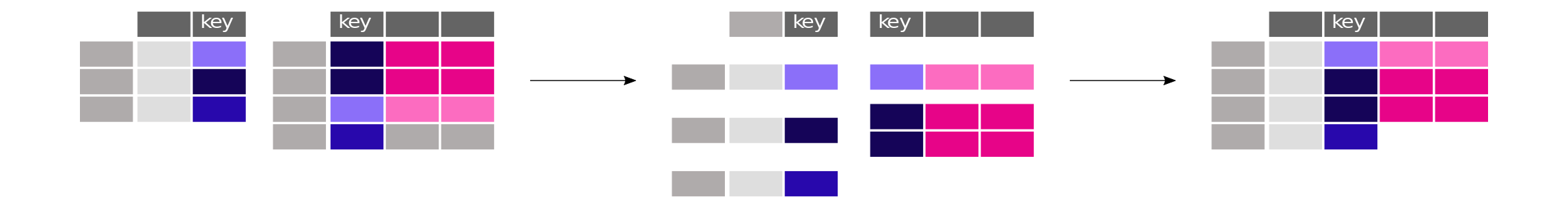
pd.merge(left, right, how='outer', left_on="key", right_on="key", suffixes=('_left', '_right'), indicator=False)
Rules for data management
1. Never ever change source data
- Source data: Original dataset as downloaded or collected
- Commit the source data to git and never change it
- All modified datasets should be stored under different names
- Modified datasets should not be under version control!
2. Separate data mgm’t and analysis
- Data management: Converting source data to formats your analysis programs need
- Separate data management code from analysis code
- Never modify the content of a variable outside the data management code!
3. Values have no internal structure
- a.k.a. the first normal form
- I.e., no need for parsing values before using them
- E.g. store first names and last names separately
- Not too often a problem in economic data
- X-digit industrial or educational classifiers
- Store each digit level you need in a separate variable
4. No redundant information in tables
- a.k.a. the second normal form
- In a panel structure: Store time-constant characteristics in a separate table
- Violations make things much harder and error-prone:
- Changes to data
- Consistency checks
- Selecting observations
5. No structure in variable names (and use meaningful names)
- a.k.a. use long format if you can
- There should not be different variables with similar content referring to different time periods etc.
- If you need wide format for regressions, still do your data management in long format