%%HTML
<link rel="stylesheet" type="text/css" href="https://raw.githubusercontent.com/malkaguillot/Foundations-in-Data-Science-and-Machine-Learning/refs/heads/main/docs/utils/custom.css">
<link rel="stylesheet" type="text/css" href="../utils/custom.css">
References
- Békés & Kézdi (2022) 13 & 14
- Introduction to Statistical Learning chap 1. & 2 & 5.1
- Kleinberg, Ludwig, Mullainathan, and Obermeyer (2015), "Prediction Policy Problems." American Economic Review, 105 (5), pp. 491-95.
- Mullainathan and Spiess (2017), "Machine Learning: An Applied Econometric Approach"), Journal of Economic Perspectives, 31 (2), pp. 87-106,
What is ML?
A concise definition by Athey (2018):
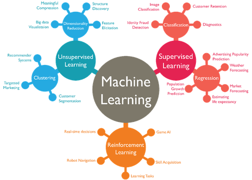
Specifically, there are three broad classifications of ML problems:
- supervised learning.
- unsupervised learning.
- reinforcement learning.
Most of the hype you hear about in recent years relates to supervised learning, and in particular, deep learning.
ML Landscape
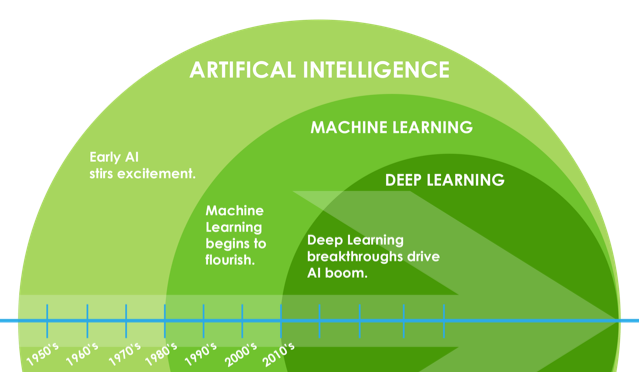
An Aside: ML and Artificial Intelligence (AI)
Unsupervised Learning
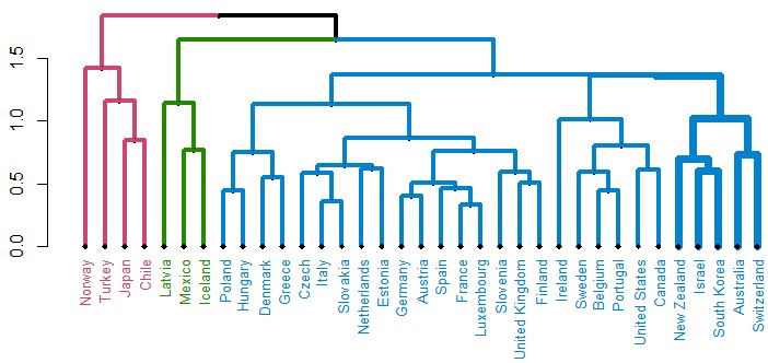
In unsupervised learning, the goal is to divide high-dimensional data into clusters that are similar in their set of features $(X)$.
Examples of algorithms:
- principal component analysis (PCA)
- $k$-means clustering
- Latent Dirichlet Allocation (LDA)
Applications:
- image recognition
- cluster analysis
- topic modelling
Reinforcement Learning (RL)
A definition by Sutton and Barto (2018):
Prominent examples:
Games (e.g., Chess, AlphaGo).
Autonomous cars.
Supervised Learning
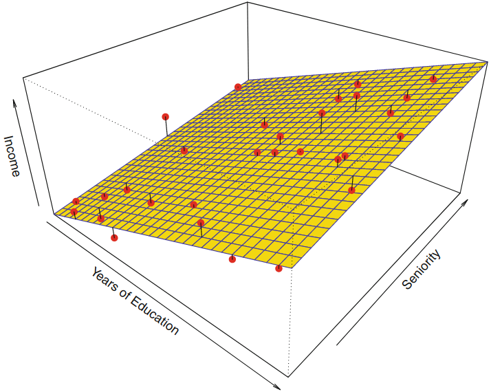
Consider the following data generating process (DGP):
$$Y=f(\boldsymbol{X})+\epsilon$$ where $Y$ is the outcome variable, $\boldsymbol{X}$ is a $1\times p$ vector of "features", and $\epsilon$ is the irreducible error.
- Training set ("in-sample"): $\\{(x_i,y_i)\\}_{i=1}^{n}$
- Test set ("out-of-sample"): $\\{(x_i,y_i)\\}_{i=n+1}^{m}$

Typical assumptions: (1) independent observations; (2) stable DGP across training and test sets.
The Goal of Supervised Learning
Use a labelled test set ($X$ and $Y$ are known) to construct $\hat{f}(X)$ such that it generalizes to unseen test set (only $X$ is known).
If $Y$ is continuous: regression problem,
- we are interested in estimating the conditional mean function $E[Y|X]$.
- Example: Predicting house prices based on their features (e.g., size, location, number of bedrooms).
If $Y$ is categorical: classification problem,
- we are interested in estimating the conditional probability function $P(Y|X)$.
- Example: Predicting whether an email is spam or not based on its content.
Supervised Learning Algorithms
ML comes with a rich set of parametric and non-parametric prediction algorithms (approximate year of discovery in parenthesis):
- Linear and logistic regression (1805, 1958).
- Decision and regression trees (1984).
- K-Nearest neighbors (1967).
- Support vector machines (1990s).
- Neural networks (1940s, 1970s, 1980s, 1990s).
- Simulation methods (Random forests (2001), bagging (2001), boosting (1990)).
- etc.
Supervised ML Workflow
Step 1: Define the Prediction Task - Pre-processing of the features
- Decompose the observations in test/training set
Step 2: Explore the Data Step 3: Choose the Model Cross-Validation Strategy Step 4: Hyperparameter Tuning with Cross-Validationn - Assess the validity of the model
- Select the best parameters
Step 5: Train the Final Model with Best Hyperparameters on the Train Set Step 6: Evaluate the Model on the Holdout Test set - Training the best model on the training set and evaluate the model using the test set
Step 7: (Deploy the Model)
Step 1: Define the Prediction Task
Boston housing data
We will use the Boston housing data: housing data for 506 census tracts of Boston from the 1970 census (Harrison and Rubinfeld, 1978).
The sample is available from sklearn and contains :
- 13 attributes of housing markets around Boston
population.
medv(target): median value of owner-occupied homes in USD 1000's.lstat(predictor): percentage of lower status of the
chas(predictor): Charles River dummy variable (= 1 if tract bounds river; 0 otherwise).
- 506 entries: aggregated data for homes from various suburbs in Boston, Massachusetts.
Objective: predict the value of prices medv of the house using the given features
Set up and load data
import numpy as np
import pandas as pd
# import patsy

from sklearn.preprocessing import StandardScaler, OneHotEncoder
from sklearn.model_selection import GridSearchCV, KFold, train_test_split
from sklearn.linear_model import LogisticRegression, LogisticRegressionCV
from sklearn.pipeline import Pipeline
from sklearn.metrics import roc_curve, roc_auc_score, classification_report, accuracy_score, confusion_matrix

import seaborn as sns
import matplotlib.pyplot as plt
df = pd.read_csv("../../data/BostonHousing.csv")
The data contain the following variables:
| Variable | Description |
|---|---|
| CRIM | per capita crime rate by town |
| ZN | proportion of residential land zoned for lots over 25,000 sq.ft. |
| INDUS | proportion of non-retail business acres per town |
| CHAS | Charles River dummy variable (= 1 if tract bounds river; 0 otherwise) |
| NOX | nitric oxides concentration (parts per 10 million) |
| RM | average number of rooms per dwelling |
| AGE | proportion of owner-occupied units built prior to 1940 |
| DIS | weighted distances to five Boston employment centres |
| RAD | index of accessibility to radial highways |
| TAX | full-value property-tax rate per $10,000 |
| PTRATIO | pupil-teacher ratio by town |
| B | 1000(Bk - 0.63)^2 where Bk is the proportion of black people by town |
| LSTAT | % lower status of the population |
df.describe()
| crim | zn | indus | chas | nox | rm | age | dis | rad | tax | ptratio | b | lstat | medv | |
|---|---|---|---|---|---|---|---|---|---|---|---|---|---|---|
| count | 506.000000 | 506.000000 | 506.000000 | 506.000000 | 506.000000 | 506.000000 | 506.000000 | 506.000000 | 506.000000 | 506.000000 | 506.000000 | 506.000000 | 506.000000 | 506.000000 |
| mean | 3.613524 | 11.363636 | 11.136779 | 0.069170 | 0.554695 | 6.284634 | 68.574901 | 3.795043 | 9.549407 | 408.237154 | 18.455534 | 356.674032 | 12.653063 | 22.532806 |
| std | 8.601545 | 23.322453 | 6.860353 | 0.253994 | 0.115878 | 0.702617 | 28.148861 | 2.105710 | 8.707259 | 168.537116 | 2.164946 | 91.294864 | 7.141062 | 9.197104 |
| min | 0.006320 | 0.000000 | 0.460000 | 0.000000 | 0.385000 | 3.561000 | 2.900000 | 1.129600 | 1.000000 | 187.000000 | 12.600000 | 0.320000 | 1.730000 | 5.000000 |
| 25% | 0.082045 | 0.000000 | 5.190000 | 0.000000 | 0.449000 | 5.885500 | 45.025000 | 2.100175 | 4.000000 | 279.000000 | 17.400000 | 375.377500 | 6.950000 | 17.025000 |
| 50% | 0.256510 | 0.000000 | 9.690000 | 0.000000 | 0.538000 | 6.208500 | 77.500000 | 3.207450 | 5.000000 | 330.000000 | 19.050000 | 391.440000 | 11.360000 | 21.200000 |
| 75% | 3.677083 | 12.500000 | 18.100000 | 0.000000 | 0.624000 | 6.623500 | 94.075000 | 5.188425 | 24.000000 | 666.000000 | 20.200000 | 396.225000 | 16.955000 | 25.000000 |
| max | 88.976200 | 100.000000 | 27.740000 | 1.000000 | 0.871000 | 8.780000 | 100.000000 | 12.126500 | 24.000000 | 711.000000 | 22.000000 | 396.900000 | 37.970000 | 50.000000 |
Create $X$ and $y$
X_full=df.drop('medv', axis=1)
y_full= df['medv']

n_samples = X_full.shape[0]
n_features = X_full.shape[1]
print(n_samples, n_features)
506 13
X_full.head()
| crim | zn | indus | chas | nox | rm | age | dis | rad | tax | ptratio | b | lstat | |
|---|---|---|---|---|---|---|---|---|---|---|---|---|---|
| 0 | 0.00632 | 18.0 | 2.31 | 0 | 0.538 | 6.575 | 65.2 | 4.0900 | 1 | 296 | 15.3 | 396.90 | 4.98 |
| 1 | 0.02731 | 0.0 | 7.07 | 0 | 0.469 | 6.421 | 78.9 | 4.9671 | 2 | 242 | 17.8 | 396.90 | 9.14 |
| 2 | 0.02729 | 0.0 | 7.07 | 0 | 0.469 | 7.185 | 61.1 | 4.9671 | 2 | 242 | 17.8 | 392.83 | 4.03 |
| 3 | 0.03237 | 0.0 | 2.18 | 0 | 0.458 | 6.998 | 45.8 | 6.0622 | 3 | 222 | 18.7 | 394.63 | 2.94 |
| 4 | 0.06905 | 0.0 | 2.18 | 0 | 0.458 | 7.147 | 54.2 | 6.0622 | 3 | 222 | 18.7 | 396.90 | 5.33 |
Look for NA values in the dataset
X_full.isna().sum()
crim       0
zn         0
indus      0
chas       0
nox        0
rm         0
age        0
dis        0
rad        0
tax        0
ptratio    0
b          0
lstat      0
dtype: int64
There is none
Step 2: Exploratory Data Analysis
Quantity to predict= price (target or $y$)
Before the regression, let us inspect the features and their distributions.
y_full.shape
(506,)
sns.set(rc={'figure.figsize':(6,4)})
plt.hist(y_full, bins=30)
plt.xlabel("House prices in $1000", size=15)
plt.ylabel('count', size=15)
plt.title('Distribution of median price in each neighborhood', size=20)
plt.show()

Features ($X$) used for prediction
X_full.shape
(506, 13)
Distributions
Histogram plots to look at the distribution
X_full.hist(bins=50, figsize=(15,10))
plt.show()

Correlations
Boston Correlation Heatmap Example with Seaborn
The seaborn package offers a heatmap that will allow a two-dimensional graphical representation of the Boston data. The heatmap will represent the individual values that are contained in a matrix are represented as colors.
import pandas as pd
import matplotlib.pyplot as plt
correlation_matrix = X_full.corr().round(2)
sns.heatmap(correlation_matrix) #annot=True
plt.show()

Check for multicolinearity
An important point in selecting features for a linear regression model is to check for multicolinearity.
The features RAD, TAX have a correlation of 0.91. These feature pairs are strongly correlated to each other. This can affect the model.
Same goes for the features DIS and AGE which have a correlation of -0.75.
Correlation plots
from pandas.plotting import scatter_matrix
scatter_matrix(X_full, figsize=(12, 8))
array([[<Axes: xlabel='crim', ylabel='crim'>,
        <Axes: xlabel='zn', ylabel='crim'>,
        <Axes: xlabel='indus', ylabel='crim'>,
        <Axes: xlabel='chas', ylabel='crim'>,
        <Axes: xlabel='nox', ylabel='crim'>,
        <Axes: xlabel='rm', ylabel='crim'>,
        <Axes: xlabel='age', ylabel='crim'>,
        <Axes: xlabel='dis', ylabel='crim'>,
        <Axes: xlabel='rad', ylabel='crim'>,
        <Axes: xlabel='tax', ylabel='crim'>,
        <Axes: xlabel='ptratio', ylabel='crim'>,
        <Axes: xlabel='b', ylabel='crim'>,
        <Axes: xlabel='lstat', ylabel='crim'>],
       [<Axes: xlabel='crim', ylabel='zn'>,
        <Axes: xlabel='zn', ylabel='zn'>,
        <Axes: xlabel='indus', ylabel='zn'>,
        <Axes: xlabel='chas', ylabel='zn'>,
        <Axes: xlabel='nox', ylabel='zn'>,
        <Axes: xlabel='rm', ylabel='zn'>,
        <Axes: xlabel='age', ylabel='zn'>,
        <Axes: xlabel='dis', ylabel='zn'>,
        <Axes: xlabel='rad', ylabel='zn'>,
        <Axes: xlabel='tax', ylabel='zn'>,
        <Axes: xlabel='ptratio', ylabel='zn'>,
        <Axes: xlabel='b', ylabel='zn'>,
        <Axes: xlabel='lstat', ylabel='zn'>],
       [<Axes: xlabel='crim', ylabel='indus'>,
        <Axes: xlabel='zn', ylabel='indus'>,
        <Axes: xlabel='indus', ylabel='indus'>,
        <Axes: xlabel='chas', ylabel='indus'>,
        <Axes: xlabel='nox', ylabel='indus'>,
        <Axes: xlabel='rm', ylabel='indus'>,
        <Axes: xlabel='age', ylabel='indus'>,
        <Axes: xlabel='dis', ylabel='indus'>,
        <Axes: xlabel='rad', ylabel='indus'>,
        <Axes: xlabel='tax', ylabel='indus'>,
        <Axes: xlabel='ptratio', ylabel='indus'>,
        <Axes: xlabel='b', ylabel='indus'>,
        <Axes: xlabel='lstat', ylabel='indus'>],
       [<Axes: xlabel='crim', ylabel='chas'>,
        <Axes: xlabel='zn', ylabel='chas'>,
        <Axes: xlabel='indus', ylabel='chas'>,
        <Axes: xlabel='chas', ylabel='chas'>,
        <Axes: xlabel='nox', ylabel='chas'>,
        <Axes: xlabel='rm', ylabel='chas'>,
        <Axes: xlabel='age', ylabel='chas'>,
        <Axes: xlabel='dis', ylabel='chas'>,
        <Axes: xlabel='rad', ylabel='chas'>,
        <Axes: xlabel='tax', ylabel='chas'>,
        <Axes: xlabel='ptratio', ylabel='chas'>,
        <Axes: xlabel='b', ylabel='chas'>,
        <Axes: xlabel='lstat', ylabel='chas'>],
       [<Axes: xlabel='crim', ylabel='nox'>,
        <Axes: xlabel='zn', ylabel='nox'>,
        <Axes: xlabel='indus', ylabel='nox'>,
        <Axes: xlabel='chas', ylabel='nox'>,
        <Axes: xlabel='nox', ylabel='nox'>,
        <Axes: xlabel='rm', ylabel='nox'>,
        <Axes: xlabel='age', ylabel='nox'>,
        <Axes: xlabel='dis', ylabel='nox'>,
        <Axes: xlabel='rad', ylabel='nox'>,
        <Axes: xlabel='tax', ylabel='nox'>,
        <Axes: xlabel='ptratio', ylabel='nox'>,
        <Axes: xlabel='b', ylabel='nox'>,
        <Axes: xlabel='lstat', ylabel='nox'>],
       [<Axes: xlabel='crim', ylabel='rm'>,
        <Axes: xlabel='zn', ylabel='rm'>,
        <Axes: xlabel='indus', ylabel='rm'>,
        <Axes: xlabel='chas', ylabel='rm'>,
        <Axes: xlabel='nox', ylabel='rm'>,
        <Axes: xlabel='rm', ylabel='rm'>,
        <Axes: xlabel='age', ylabel='rm'>,
        <Axes: xlabel='dis', ylabel='rm'>,
        <Axes: xlabel='rad', ylabel='rm'>,
        <Axes: xlabel='tax', ylabel='rm'>,
        <Axes: xlabel='ptratio', ylabel='rm'>,
        <Axes: xlabel='b', ylabel='rm'>,
        <Axes: xlabel='lstat', ylabel='rm'>],
       [<Axes: xlabel='crim', ylabel='age'>,
        <Axes: xlabel='zn', ylabel='age'>,
        <Axes: xlabel='indus', ylabel='age'>,
        <Axes: xlabel='chas', ylabel='age'>,
        <Axes: xlabel='nox', ylabel='age'>,
        <Axes: xlabel='rm', ylabel='age'>,
        <Axes: xlabel='age', ylabel='age'>,
        <Axes: xlabel='dis', ylabel='age'>,
        <Axes: xlabel='rad', ylabel='age'>,
        <Axes: xlabel='tax', ylabel='age'>,
        <Axes: xlabel='ptratio', ylabel='age'>,
        <Axes: xlabel='b', ylabel='age'>,
        <Axes: xlabel='lstat', ylabel='age'>],
       [<Axes: xlabel='crim', ylabel='dis'>,
        <Axes: xlabel='zn', ylabel='dis'>,
        <Axes: xlabel='indus', ylabel='dis'>,
        <Axes: xlabel='chas', ylabel='dis'>,
        <Axes: xlabel='nox', ylabel='dis'>,
        <Axes: xlabel='rm', ylabel='dis'>,
        <Axes: xlabel='age', ylabel='dis'>,
        <Axes: xlabel='dis', ylabel='dis'>,
        <Axes: xlabel='rad', ylabel='dis'>,
        <Axes: xlabel='tax', ylabel='dis'>,
        <Axes: xlabel='ptratio', ylabel='dis'>,
        <Axes: xlabel='b', ylabel='dis'>,
        <Axes: xlabel='lstat', ylabel='dis'>],
       [<Axes: xlabel='crim', ylabel='rad'>,
        <Axes: xlabel='zn', ylabel='rad'>,
        <Axes: xlabel='indus', ylabel='rad'>,
        <Axes: xlabel='chas', ylabel='rad'>,
        <Axes: xlabel='nox', ylabel='rad'>,
        <Axes: xlabel='rm', ylabel='rad'>,
        <Axes: xlabel='age', ylabel='rad'>,
        <Axes: xlabel='dis', ylabel='rad'>,
        <Axes: xlabel='rad', ylabel='rad'>,
        <Axes: xlabel='tax', ylabel='rad'>,
        <Axes: xlabel='ptratio', ylabel='rad'>,
        <Axes: xlabel='b', ylabel='rad'>,
        <Axes: xlabel='lstat', ylabel='rad'>],
       [<Axes: xlabel='crim', ylabel='tax'>,
        <Axes: xlabel='zn', ylabel='tax'>,
        <Axes: xlabel='indus', ylabel='tax'>,
        <Axes: xlabel='chas', ylabel='tax'>,
        <Axes: xlabel='nox', ylabel='tax'>,
        <Axes: xlabel='rm', ylabel='tax'>,
        <Axes: xlabel='age', ylabel='tax'>,
        <Axes: xlabel='dis', ylabel='tax'>,
        <Axes: xlabel='rad', ylabel='tax'>,
        <Axes: xlabel='tax', ylabel='tax'>,
        <Axes: xlabel='ptratio', ylabel='tax'>,
        <Axes: xlabel='b', ylabel='tax'>,
        <Axes: xlabel='lstat', ylabel='tax'>],
       [<Axes: xlabel='crim', ylabel='ptratio'>,
        <Axes: xlabel='zn', ylabel='ptratio'>,
        <Axes: xlabel='indus', ylabel='ptratio'>,
        <Axes: xlabel='chas', ylabel='ptratio'>,
        <Axes: xlabel='nox', ylabel='ptratio'>,
        <Axes: xlabel='rm', ylabel='ptratio'>,
        <Axes: xlabel='age', ylabel='ptratio'>,
        <Axes: xlabel='dis', ylabel='ptratio'>,
        <Axes: xlabel='rad', ylabel='ptratio'>,
        <Axes: xlabel='tax', ylabel='ptratio'>,
        <Axes: xlabel='ptratio', ylabel='ptratio'>,
        <Axes: xlabel='b', ylabel='ptratio'>,
        <Axes: xlabel='lstat', ylabel='ptratio'>],
       [<Axes: xlabel='crim', ylabel='b'>,
        <Axes: xlabel='zn', ylabel='b'>,
        <Axes: xlabel='indus', ylabel='b'>,
        <Axes: xlabel='chas', ylabel='b'>,
        <Axes: xlabel='nox', ylabel='b'>,
        <Axes: xlabel='rm', ylabel='b'>,
        <Axes: xlabel='age', ylabel='b'>,
        <Axes: xlabel='dis', ylabel='b'>,
        <Axes: xlabel='rad', ylabel='b'>,
        <Axes: xlabel='tax', ylabel='b'>,
        <Axes: xlabel='ptratio', ylabel='b'>,
        <Axes: xlabel='b', ylabel='b'>,
        <Axes: xlabel='lstat', ylabel='b'>],
       [<Axes: xlabel='crim', ylabel='lstat'>,
        <Axes: xlabel='zn', ylabel='lstat'>,
        <Axes: xlabel='indus', ylabel='lstat'>,
        <Axes: xlabel='chas', ylabel='lstat'>,
        <Axes: xlabel='nox', ylabel='lstat'>,
        <Axes: xlabel='rm', ylabel='lstat'>,
        <Axes: xlabel='age', ylabel='lstat'>,
        <Axes: xlabel='dis', ylabel='lstat'>,
        <Axes: xlabel='rad', ylabel='lstat'>,
        <Axes: xlabel='tax', ylabel='lstat'>,
        <Axes: xlabel='ptratio', ylabel='lstat'>,
        <Axes: xlabel='b', ylabel='lstat'>,
        <Axes: xlabel='lstat', ylabel='lstat'>]], dtype=object)

Scatter plot relative to the target (price)
(X_full.columns)
Index(['crim', 'zn', 'indus', 'chas', 'nox', 'rm', 'age', 'dis', 'rad', 'tax',
       'ptratio', 'b', 'lstat'],
      dtype='object')
fig, axs= plt.subplots(3, 5, figsize=(20, 12))
i=0
for ax in axs.flat:
    if i<len(X_full.columns):
        feature_name = X_full.columns[i]
        ax.scatter(X_full[feature_name], y_full, alpha=0.1)
        ax.set(xlabel=feature_name, ylabel='Price')
        i=i+1

What can we say ?
The prices increase as the value of RM increases linearly. There are few outliers and the data seems to be capped at 50.
The prices tend to decrease with an increase in LSTAT. Though it doesn’t look to be following exactly a linear line.
Linear Regression as a predictive model
Model building
Deciding about the predictors to include in the model and their functional form.
We have strong computers, cloud, etc - why could not we try out all possible models and pick the best one?
- Too many models possible!
2 methods to build models:
- By hand -- mix domain knowledge and statistics
- By Smart algorithms $=$ machine learning
Linear Regression
$$Y=\beta_0 + \beta_1 X_1 + \cdots + \beta_p X_p + \epsilon $$
$=$ one of the simplest algorithms for doing supervised learning
A good starting point before studying more complex learning methods
Interpretation of $\beta_j$ = the average effect on $Y$ of a unit increase in $X_j$ holding all other predictors fixed
Linear estimate
Linear Models: pros and cons
Core ML concepts
Overfitting: Low Bias, High Variance
The model: high-degree polynomial
$$Y_i = \beta_0+\sum_{j=1}^{\lambda}\beta_jX_i^{\lambda}+\varepsilon_i$$
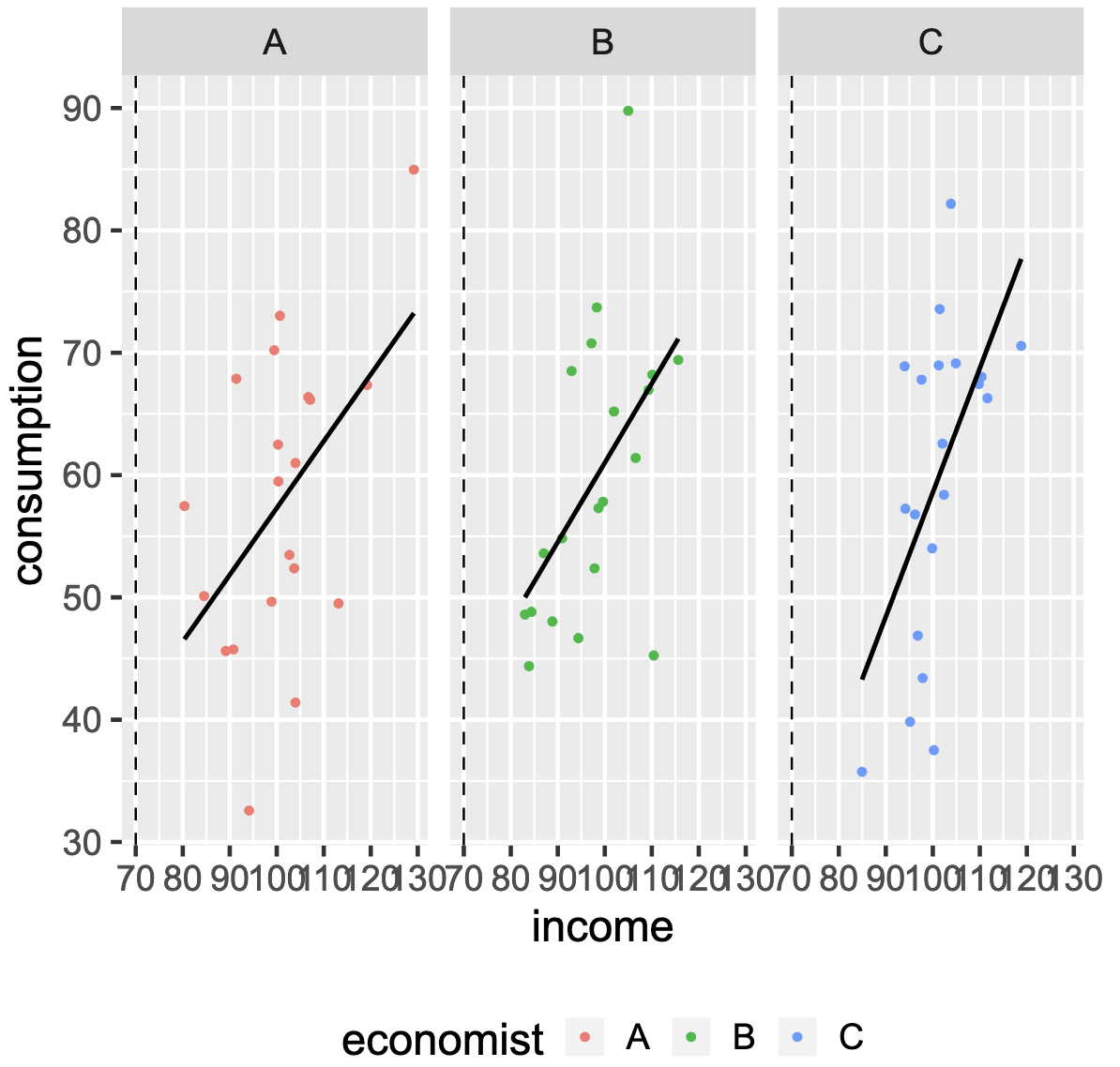
"Justfitting": Bias and Variance are Just Right
The model: linear regression
$$Y_i = \beta_0+\beta_1 X_i + \varepsilon_i$$
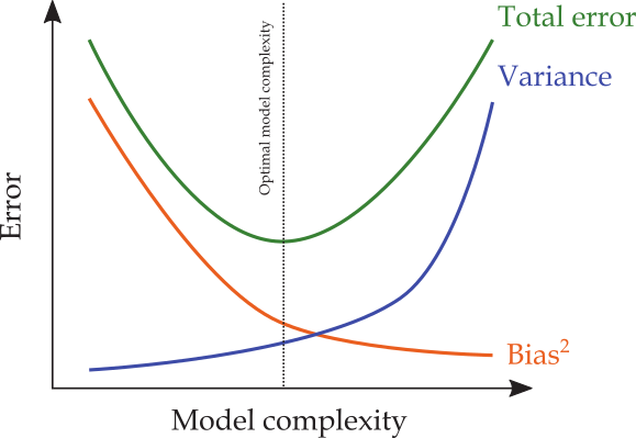
The Typical Bias-Variance Trade-off in ML
Typically, ML models strive to find levels of bias and variance that are "just right":
When is the Bias-Variance Trade-off Important?
In low-dimensional settings ( $n\gg p$ )
- overfitting is highly unlikely
- training MSE closely approximates test MSE
- conventional tools (e.g., OLS) will perform well on a test set
INTUITION: As $n\rightarrow\infty$, insignificant terms will converge to their true value (zero).
In high-dimensional settings ( $n\ll p$ )
- overfitting is highly likely
- training MSE poorly approximates test MSE
- conventional tools tend to overfit
$n\ll p$ is prevalent in big-data
Measuring the Performance of a Model using Mean Squared Error (MSE)
$$MSE= \frac{1}{n} \sum_{i=1}^n (y_i - \hat f(x_i))^2$$
- Regression setting: the
mean squared error is a metric of how well a model fits the data.
MSE will be small if the predicted responses are very close to the true responses,and will be large if for some of the observations, the predicted and true responses differ substantially
= Aggregated measure of the errors
Avoiding Overfitting: train/test split
<table>
<tr>
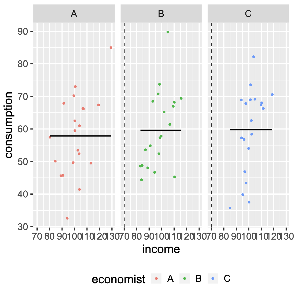
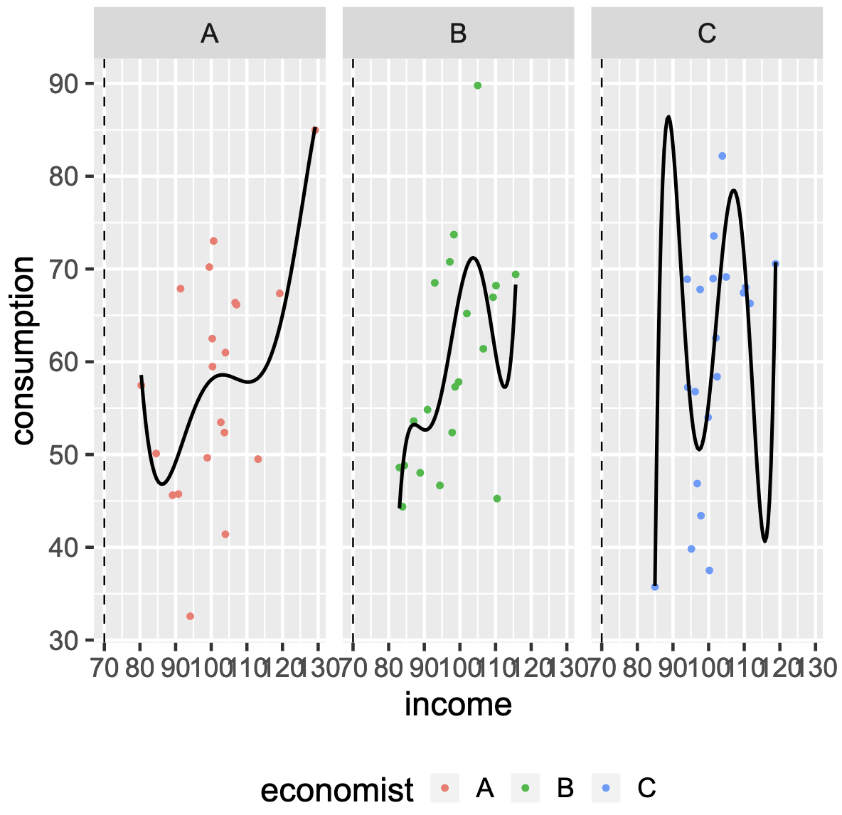
<td>3 simulated models</td>
<td><span style="color: grey;">train set MSE</span> and <span style="color: red;">test set MSE</span></td>
</tr>
</table>
%%HTML
<div style="text-align: center;"> style="text-align: center;">
    <table>
            <td>3 simulated models</td>
            <td> Flexibility:<span style="color: grey;">train set MSE</span> and <span style="color: red;">test set MSE</span></td>
        </tr>
    </table>
</div>
Training MSE, test MSE and model flexibility
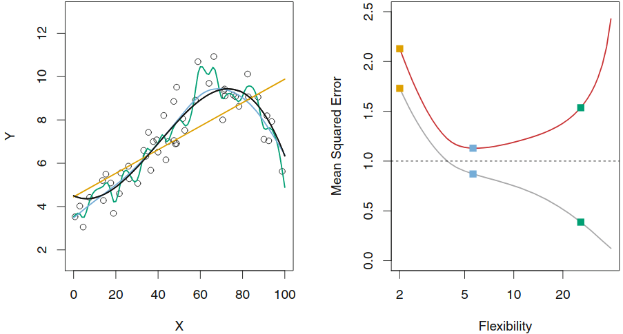
| 3 simulated models and DGP in black | Flexibility:train set MSE and test set MSE |
Increasing model flexibility tends to
Overfitting
As model flexibility increases, training MSE will decrease, but the test MSE may not.
When a given method yields a small training MSE but a large test MSE, we are said to be overfitting the data.
(We almost always expect the training MSE to be smaller than the test MSE)
Estimating test MSE is important, but requires training data...
Regularization methods
Context: Generalization of the Linear Models
Regularized fitting : ridge regression and lassoNon-linearity : nearest neighbor methodsInteractions : Tree-based methods, random forests and boosting
Why Regularization?
Key question: which features to enter into model, how to select?
- There is room for an automatic selection process.
Solution against
overfitting Allow High-Dimensional Predictors
- $p>>n$: OLS no longer has a unique solution
- $x_i$ "high-dimensional" i.e. very many regressors
- pixels on a picture
Notes: Corollary of regularization:
- Prediction Accuracy:especially when $p > n$, to control the variance
Adding a Regularization Term to the Loss Function $L(.)$
$$ \hat \beta =arg min_\beta \frac{1}{n} \sum_{i=1}^n L(h(x_i, \beta), y_i) +\lambda R(\beta) $$
$R(\beta)$ =
regularization function - $R(\beta)=\sum_{i=1}^n p(\beta_i)$ for $p(.)$ the penalty function
- measures the
expressiveness of the model
As the number of features grows, linear models become more expressive.
$\lambda$ is a
hyperparameter where higher values increase regularization
Notation: Norms
Suppose $\boldsymbol{\beta}$ is a $p\times 1$ vector with typical element $\beta_i$.
The $\ell_0$-norm is defined as $\lVert\boldsymbol{\beta}\rVert_0 = \sum_{j=1}^p \boldsymbol{1}\\{\beta_j \neq 0\\}$,
- i.e., the number of non-zero elements in $\boldsymbol{\beta}$.
The $\ell_1$-norm is defined as $\lVert\boldsymbol{\beta}\rVert_1=\sum_{j=1}^{p}|\beta_j|$.
The $\ell_2$-norm is defined as $\lVert\boldsymbol{\beta}\rVert_2=\left(\sum_{j=1}^{p}|\beta_j|^2\right)^{\frac{1}{2}}$
- i.e., Euclidean norm.
Commonly used penalty functions
Regularization problem:
$$\underset{\beta_{0}, \beta}{\operatorname{min}} \sum_{i=1}^{N}\left(y_{i}-\beta_{0}-\sum_{j=1}^{p} x_{i j} \beta_{j}\right)^{2}+\lambda R(\beta)$$
| Method | $R(\boldsymbol{\beta})$ |
|---|---|
| 0 | |
| $\lVert\boldsymbol{\beta}\rVert_0$ | |
| $\lVert\boldsymbol{\beta}\rVert_1$ | |
| $\lVert\boldsymbol{\beta}\rVert_2^2$ | |
| $\alpha\lVert\boldsymbol{\beta}\rVert_1 + (1-\alpha)\lVert\boldsymbol{\beta}\rVert_2^2$ |
Prerequisite: centering and scaling
In what follows, we assume that each feature is centered and scaled to have mean zero and unit variance, as follows:
$$\frac{x_{ij} - \widehat\mu_i}{\widehat\sigma_{i}}, \qquad\text{for }j=1,2, \ldots, p$$
where $\widehat\mu_i$ and $\widehat\sigma_i$ are the estimated mean and standard deviation of $x_i$ estimated over the training set.
Remark: This is not important when using OLS (why?)
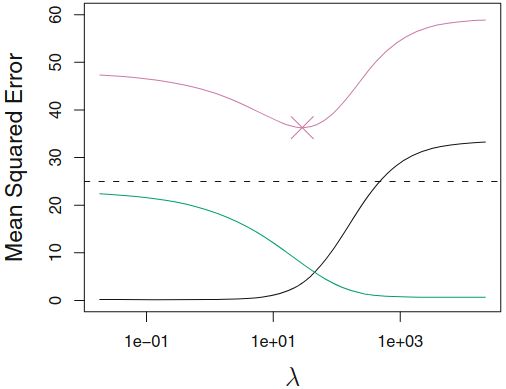
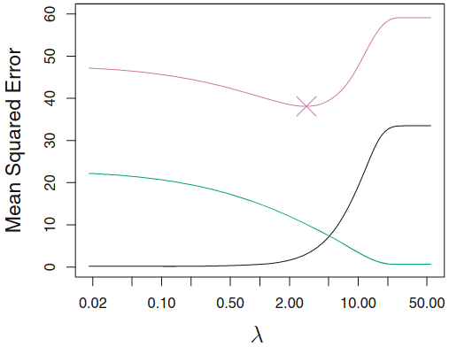
Ridge Regression
$$\min_{\beta} \sum_{i=1}^n \left(y_i - \beta_{0}-\sum_{j=1}^{p} x_{i j} \beta_{j} \right)^2 + \lambda \sum_{j=1}^p \beta_j^2 $$
Where
- $\lambda > 0$ = penalty parameter
- covariates can be high-dimensionnal $p>>N$
Trade-off, from the minimization of the sum of
- RSS
- shrinkage penalty: decreases with $\beta_j$
$\rightarrow$ relative importance given by $\lambda$
Ridge Regression: shrinkage to $0$
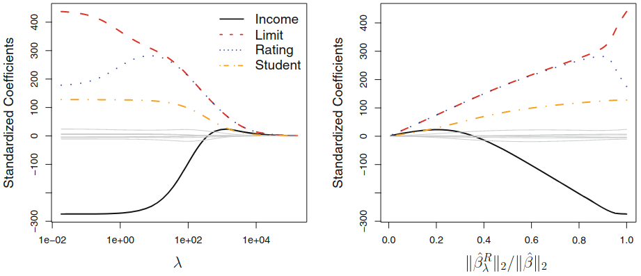
Ridge vs. Linear Models
- when outcome and predictors are close to having a linear relationship, the OLS will have low bias but potentially high variance
- small change in the training data $\rightarrow$ large change in the estimates
- worse with $p$ close tp $n$
- if $p>n$, OLS do not have a unique solution
$\rightarrow$ ridge regression works best in situations where the least squares estimates have high variance
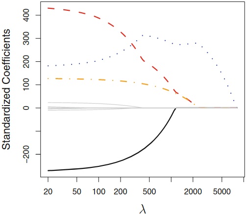
LASSO (Least Absolute Shrinkage and Selection Operator)
LASSO proposes a method to build a model which just
Modifies the way regression coefficients are estimated by adding a penalty term for too many coefficients
Notes: Ridge: the penalty shinks coefficients toward $0$ but not exactly to $0$
This may not be a problem for prediction accuracy, but it can create a challenge in model interpretation when $p$ is quite large
Lasso
$$ \hat \beta =arg min_\beta \frac{1}{n} \sum_{i=1}^n \left( y_i -(\beta_0 + \sum_{j=1}^k\beta_jx_{ij})\right)^2 +\lambda \sum_{j=1}^k |\beta_j| $$
$R(\beta)= \sum_{j=1}^k |\beta_j|=$
regularization function with a $\ell_1$-norm penalty function$\lambda$ is a
hyperparameter (or tunning) where higher values increase regularization
Notes:
- Lasso automatically performs feature selection and outputs a sparse model.
Lasso Coefficients
Constrained Regression
The minimization problem can be written as follow:
$$ \sum_{i=1}^n(y_i-x_i'\beta)^2 \textrm{ s.t. } \sum_{j=1}^p p(\beta_j) \leq s,$$
Where
- Ridge: $\sum_{j=1}^p \beta_j^2 <s $
$\rightarrow$ equation of a
circle - Lasso: $\sum_{j=1}^p |\beta_j| <s $
$\rightarrow$ equation of a
diamond
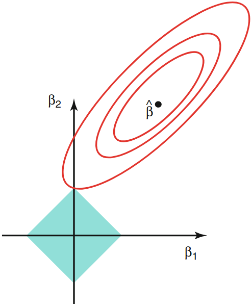
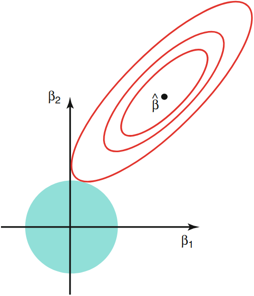
Constraint Regions: Lasso vs. ridge
Contours of the error and constraint functions for lasso (left) and ridge (right).
- The solid blue areas are the constraint regions, $\beta_{1}^{2}+\beta_{2}^{2} \leq \lambda,$ and $|\beta_{1}|+|\beta_{2}| \leq \lambda$
- the red ellipses are the contours of the RSS and $\widehat\beta$ is the OLS estimator.
| Lasso | Ridge |
|---|---|
 |
 |
Elastic Net = Lasso + Ridge
$$ MSE(\beta)+\lambda_1 \sum_{j=1}^p |\beta_j| +\lambda_2 \sum_{j=1}^p \beta_j^2$$
$\lambda_1$, $\lambda_2$ $=$ strength of $\ell_1$-norm (Lasso) penalty and $\ell_2^2$-norm (Ridge) penalty
Selecting Elastic Net Hyperparameters
Elastic net
hyperparameters should be selected to optimize out-of-sample fit (measured by mean squared error or MSE).“Grid search” - scans over the hyperparameter space ($\lambda_1 \geq 0, \lambda_2\geq 0$),
- computes out-of-sample MSE for all pairs $(\lambda_1, \lambda_2)$ ,
- selects the MSE-minimizing model.
Feature Engineering
2 extensions of the Linear Model
Going further model's assumptions:
the additive: the effect of changes in a predictor $X_j$ on the response $Y$ is independent of the values of the other predictors
linearity: the change in the response $Y$ due to a one-unit change in $X_j$ is constant
Non Linearity
- Include transformed versions of the predictors in the model
$\Rightarrow$ Including polynomials in $X$ may provide a better fit
Scikit-Learn Design Overview
Transformer (preprocessor): An object that transforms a data set.
- e.g.
preprocessing.StandardScaler - Transformation is performed by the
transform()method.
Estimator: an object that can estimate parameters
- e.g.
linear_models.LinearRegression - Estimation performed by
fit()method - Exogenous parameters (provided by the researcher) are called
hyperparameters - The convenience method
fit_transform()both fits an estimator and returns the transformed input data set.
Predictor: An object that forms a prediction from an input data set.
- e.g.
LinearRegression, after training - The
predict()method forms the predictions. - It also has a
score()method that measures the quality of the predictions given a test set.
Step 3: set, train and evaluate the model
Data cleaning
The missing features should be either:
- dropped
- imputed to some value (zero, the mean, the median...)
Drop the observations with price >=50 (because of the right censure)
mask=y_full<50

y_full=y_full[mask==True]
X_full=X_full[mask==True]
Prepare Training and Test Sets using train_test_split
Pure ramdomness of the sampling method
from sklearn.model_selection import train_test_split

X_train, X_test, y_train, y_test = train_test_split(X_full, y_full,test_size=0.2, random_state=1)

print("train data", X_train.shape, y_train.shape)
print("test data", X_test.shape,  y_test.shape)
train data (392, 13) (392,)
test data (98, 13) (98,)
Feature Scaling
Most common scaling methods:
- standardization= normalization by substracting the mean and dividing by the standard deviation (values are not bounded)
$x_1^{scaled} = \frac{x^1 - \bar x_1 }{sd(x^1)}$
- Min-max scaling= normalization by substracting the minimum and dividing by the maximum (values between
0and1)
from sklearn.preprocessing import StandardScaler, MinMaxScaler

scaler = StandardScaler().fit(X_train)
X_train_scaled = scaler.transform(X_train)
X_test_scaled = scaler.transform(X_test)
Select and Train a Model
Regression algorithm (we consider firs the LinearRegression, more algorithms will be discussed later):
# our first machine learning model
from sklearn.linear_model import LinearRegression
lin_reg = LinearRegression()
lin_reg
LinearRegression()In a Jupyter environment, please rerun this cell to show the HTML representation or trust the notebook.
On GitHub, the HTML representation is unable to render, please try loading this page with nbviewer.org.
LinearRegression()
lin_reg.fit(X_train_scaled, y_train)
LinearRegression()In a Jupyter environment, please rerun this cell to show the HTML representation or trust the notebook.
On GitHub, the HTML representation is unable to render, please try loading this page with nbviewer.org.
LinearRegression()
print("R-squared for training dataset:{}".
      format(np.round(lin_reg.score(X_train_scaled, y_train), 2)))
R-squared for training dataset:0.79
print("R-squared for test dataset:{}".
      format(np.round(lin_reg.score(X_test_scaled, y_test), 2)))
R-squared for test dataset:0.73
Note: $R^2 =$ the proportion of variance (of $y$) that has been explained by the independent variables in the model.
Coefficients of the linear regression
lin_reg.coef_
array([-0.82250959,  0.96267645, -0.54388693,  0.187684  , -1.50325117,
        2.15830284, -0.54795352, -2.78522878,  2.16616351, -2.21708013,
       -1.8582422 ,  0.71805978, -2.70105292])
print('The coefficients of the features from the linear model:')
print(dict(zip(features, [round(x, 2) for x in lin_reg.coef_])))
The coefficients of the features from the linear model:
{'crim': -0.82, 'zn': 0.96, 'indus': -0.54, 'chas': 0.19, 'nox': -1.5, 'rm': 2.16, 'age': -0.55, 'dis': -2.79, 'rad': 2.17, 'tax': -2.22, 'ptratio': -1.86, 'b': 0.72, 'lstat': -2.7}
Choose the best model with cross-validation
k-fold Cross-validation
Split the training set into $k$ roughly equal-sized parts ( $k=5$ in this example):
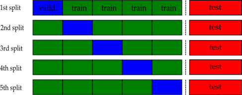
Approximate the test-MSE using the mean of $k$ split-MSEs
$$\text{CV-MSE} = \frac{1}{k}\sum_{j=1}^{k}\text{MSE}_j$$
Step 4: Cross-validation
K-Fold CV
from sklearn.model_selection import cross_val_score, cross_val_predict
from sklearn.model_selection import KFold
# Perform 5-fold cross validation
scores = cross_val_score(lin_reg, X_train_scaled, y_train,
                         scoring="neg_mean_squared_error", # evaluation metrics
                         cv=5)
scores
array([ -7.74021081, -15.46731828, -14.72344763, -17.14433289,
       -18.96092531])
# the other way of doing the same thing (more explicit)

# create a KFold object with 5 splits
folds = KFold(n_splits = 5, shuffle = True, random_state = 100)
scores = cross_val_score(lin_reg, X_train_scaled, y_train, scoring='neg_mean_squared_error', cv=folds)
scores
array([-18.32023985, -11.84760498, -17.04867667, -16.44238641,
       -10.9874587 ])
Hyperparameter Tuning Using Grid Search Cross-Validation
A common use of cross-validation is for tuning hyperparameters of a model. The most common technique is what is called grid search cross-validation.
# 1. create a cross-validation scheme
from sklearn.model_selection import KFold
kfold = KFold(n_splits=10,random_state=2, shuffle=True)
kfold
KFold(n_splits=10, random_state=2, shuffle=True)
# 2. specify range of hyperparameters to tune
param_grid = [
  {'alpha': [0.0001, 0.001, 0.01, 0.1 ,1, 10],
      'l1_ratio':[.1,.5,.9,1]}
]
from sklearn.model_selection import GridSearchCV
# 3. perform grid search
# 3.1 specify model
from sklearn.linear_model import ElasticNet
elastic_net = ElasticNet()
# 3.2 call GridSearchCV()

# train across 5 folds, that's a total of (12+6)*5=90 rounds of training
model_cv = GridSearchCV(elastic_net, param_grid, cv=kfold,
                           scoring='neg_mean_squared_error',
                           return_train_score=True)
model_cv
GridSearchCV(cv=KFold(n_splits=10, random_state=2, shuffle=True),
             estimator=ElasticNet(),
             param_grid=[{'alpha': [0.0001, 0.001, 0.01, 0.1, 1, 10],
                          'l1_ratio': [0.1, 0.5, 0.9, 1]}],
             return_train_score=True, scoring='neg_mean_squared_error')
In a Jupyter environment, please rerun this cell to show the HTML representation or trust the notebook. On GitHub, the HTML representation is unable to render, please try loading this page with nbviewer.org.
GridSearchCV(cv=KFold(n_splits=10, random_state=2, shuffle=True),
             estimator=ElasticNet(),
             param_grid=[{'alpha': [0.0001, 0.001, 0.01, 0.1, 1, 10],
                          'l1_ratio': [0.1, 0.5, 0.9, 1]}],
return_train_score=True, scoring='neg_mean_squared_error')ElasticNet()
ElasticNet()
# fit the model
model_cv.fit(X_train_scaled, y_train)
GridSearchCV(cv=KFold(n_splits=10, random_state=2, shuffle=True),
             estimator=ElasticNet(),
             param_grid=[{'alpha': [0.0001, 0.001, 0.01, 0.1, 1, 10],
                          'l1_ratio': [0.1, 0.5, 0.9, 1]}],
             return_train_score=True, scoring='neg_mean_squared_error')
In a Jupyter environment, please rerun this cell to show the HTML representation or trust the notebook. On GitHub, the HTML representation is unable to render, please try loading this page with nbviewer.org.
GridSearchCV(cv=KFold(n_splits=10, random_state=2, shuffle=True),
             estimator=ElasticNet(),
             param_grid=[{'alpha': [0.0001, 0.001, 0.01, 0.1, 1, 10],
                          'l1_ratio': [0.1, 0.5, 0.9, 1]}],
return_train_score=True, scoring='neg_mean_squared_error')ElasticNet(alpha=0.01, l1_ratio=0.1)
ElasticNet(alpha=0.01, l1_ratio=0.1)
# cv results
cv_results = pd.DataFrame(model_cv.cv_results_)
cv_results.head()
| mean_fit_time | std_fit_time | mean_score_time | std_score_time | param_alpha | param_l1_ratio | params | split0_test_score | split1_test_score | split2_test_score | ... | split2_train_score | split3_train_score | split4_train_score | split5_train_score | split6_train_score | split7_train_score | split8_train_score | split9_train_score | mean_train_score | std_train_score | |
|---|---|---|---|---|---|---|---|---|---|---|---|---|---|---|---|---|---|---|---|---|---|
| 0 | 0.004507 | 0.005245 | 0.001400 | 0.002163 | 0.0001 | 0.1 | {'alpha': 0.0001, 'l1_ratio': 0.1} | -13.406530 | -14.328648 | -12.011451 | ... | -13.755289 | -13.819750 | -13.797527 | -13.206681 | -13.885470 | -11.411172 | -13.730520 | -13.507182 | -13.428291 | 0.698492 |
| 1 | 0.000864 | 0.000134 | 0.000324 | 0.000040 | 0.0001 | 0.5 | {'alpha': 0.0001, 'l1_ratio': 0.5} | -13.408003 | -14.328863 | -12.011969 | ... | -13.755289 | -13.819749 | -13.797526 | -13.206680 | -13.885470 | -11.411172 | -13.730519 | -13.507181 | -13.428290 | 0.698492 |
| 2 | 0.001147 | 0.000544 | 0.000569 | 0.000521 | 0.0001 | 0.9 | {'alpha': 0.0001, 'l1_ratio': 0.9} | -13.409477 | -14.329080 | -12.012521 | ... | -13.755288 | -13.819749 | -13.797526 | -13.206680 | -13.885469 | -11.411171 | -13.730518 | -13.507181 | -13.428289 | 0.698492 |
| 3 | 0.000787 | 0.000105 | 0.000324 | 0.000050 | 0.0001 | 1.0 | {'alpha': 0.0001, 'l1_ratio': 1} | -13.409844 | -14.329135 | -12.012652 | ... | -13.755288 | -13.819749 | -13.797525 | -13.206680 | -13.885469 | -11.411171 | -13.730518 | -13.507181 | -13.428289 | 0.698492 |
| 4 | 0.000756 | 0.000107 | 0.000287 | 0.000008 | 0.0010 | 0.1 | {'alpha': 0.001, 'l1_ratio': 0.1} | -13.354994 | -14.323175 | -11.994855 | ... | -13.755485 | -13.819927 | -13.797724 | -13.206868 | -13.885637 | -11.411323 | -13.730734 | -13.507338 | -13.428476 | 0.698504 |
5 rows × 32 columns
# plotting cv results
plt.figure(figsize=(16,6))
a= 0.01
plt.plot(cv_results.loc[cv_results['param_alpha']==a,"param_l1_ratio"], cv_results[cv_results['param_alpha']==a]["mean_test_score"])
plt.plot(cv_results.loc[cv_results['param_alpha']==a,"param_l1_ratio"], cv_results[cv_results['param_alpha']==a]["mean_train_score"])
plt.xlabel('L1 ratio')
plt.ylabel('Negative MSE')
plt.title("Optimal L1 ratio parameter for alpha={}".format(a) )
plt.legend(['test score', 'train score'], loc='upper right')
<matplotlib.legend.Legend at 0x324e73a40>

Step 5: Best model implementation and evaluation
Now we can choose the optimal value of number of features and build a final model.
best_alpha = model_cv.best_params_['alpha']
best_l1_ratio = model_cv.best_params_['l1_ratio']
print("Best alpha: ", best_alpha,   "Best l1_ratio: ", best_l1_ratio)
Best alpha: 0.01 Best l1_ratio: 0.1
# Fit model (to the training set) with optimal alpha and l1_ratio
elastic_net = ElasticNet(alpha=best_alpha, l1_ratio=best_l1_ratio)
elastic_net.fit(X_train_scaled, y_train)
ElasticNet(alpha=0.01, l1_ratio=0.1)In a Jupyter environment, please rerun this cell to show the HTML representation or trust the notebook.
On GitHub, the HTML representation is unable to render, please try loading this page with nbviewer.org.
ElasticNet(alpha=0.01, l1_ratio=0.1)
# predict prices of X_test
y_test_pred = elastic_net.predict(X_test_scaled)
# Evaluate the model
from sklearn.metrics import mean_squared_error

test_mse = mean_squared_error(y_test, y_test_pred)
test_rmse = np.sqrt(test_mse)
print("RMSE on test data: ", test_rmse)
RMSE on test data: 3.8754693909725972
NOTE: the test set RMSE estimates the expected squared prediction error on unseen data given the best model.
MSE vs. $R^2$
MSE :
- good for comparing regression models,
- but the units depend on the outcome variable and
- $\Rightarrow$ are not interpretable
Better to use $R^2$ in the test set: same ranking as MSE but it more interpretable.