%%HTML
<link rel="stylesheet" type="text/css" href="https://raw.githubusercontent.com/malkaguillot/Foundations-in-Data-Science-and-Machine-Learning/refs/heads/main/docs/utils/custom.css">
%%HTML
<link rel="stylesheet" type="text/css" href="../utils/custom.css">

%%HTML

Foundations in Data Science and Machine Learning

Module 5b: Machine Learning - Classifications

Malka Guillot

Classification Framework

• Response/target variable $y$ is qualitative (or categorical):

  • 2 categories $\rightarrow$ binary classification

  • More than 2 categories $\rightarrow$ multi-class classification

• Features $X$:

  • can be high-dimensional

• We want to assign a class to a quantitative response

  $\rightarrow$ probability to belong to the class

• Classifier: An algorithm that maps the input data to a specific category.

• Performance measures specific to classification

Classification process

1. Model probability

   • Probability of belonging to a category $$P(y=1 \mid X)$$

2. Predict probability

   • rely on this probability to assign a class to the observation.
   • For example, we can assign the class $1$ for all observations where $P(y = 1 | x) > 0.5 $
   • But we can also select a different threshold.

3. We can make errors

   • False negative
   • False positive

Confusion Matrix

• For comparing the predictions of the fitted model to the actual classes.

• After applying a classifier to a data set with known labels Yes and No:

  		Truth
  		Negative	Positive
  Prediction	Negative	True negative (TN)	False negative (FN)
  	Positive	False positive (FP)	True positive (TP)

Note that $TP+TN+FP+TP=N$, where $N$ is the number of observations.

The confusion matrix shows the number of observations by their predicted class and actual classes.

• Correctly classified: TP & TN
• Incorrectly classified: FP & FN

Precision and Recall

• Accuracy : Proportion of rightly guessed observations

  • $ \frac{ \color{green}{\text{True Positives}} + \color{#90EE90}{\text{True Negative}}} {N}$

• Precision: accuracy of positive predictions

  • $ \frac{ \color{green}{\text{True Positives}}} {\color{green}{\text{True Positives}} + \color{orange}{\text{False Positives}}}$

  • decreases with false positives.

• Recall: proportion of true positives among all actual positives

  • $ \frac{\color{green}{\text{True Positives}}}{\color{green}{\text{True Positives}} + \color{blue}{\text{False Negatives}}}$

  • decreases with false negatives.

F1 Score

• The $F_{1}$ score provides a single combined metric it is the harmonic mean of precision and recall

  $$\begin{aligned} F_{1} &= \frac{2}{\frac{1}{\text{precision}}+\frac{1}{\text{recall}}} = 2\times\frac{\text{precision}\times\text{recall}}{\text{precision}+\text{recall}} \\\\ &= \frac{\text{Total Positives}}{\text{Total Positives}+\frac{1}{2}(\text{False Negatives}+\text{False Positives})} \end{aligned}$$

• The harmonic mean gives more weight to low values.

• The F1 score values precision and recall symmetrically.

Logistic Regression

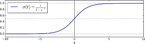
• Prediction:

$$\hat{y} = \begin{cases} 0 & \textrm{ if } \hat{p}<.5 \\\\ 1 & \textrm{ if } \hat{p}\geq.5 \end{cases} $$

Logistic Regression Cost Function

• The cost function to minimize is

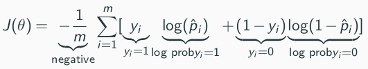
• this does not have a closed form solution

• but it is convex, so gradient descent will find the global minimum.

• Just like linear models, logistic can be regulared with L1 or L2 penalties, e.g.: $$J_{2}(\theta)=J(\theta)+\alpha_{2}\frac{1}{2}\sum_{i=1}^{n}\theta_{i}^{2}$$

Implementation of the logistic regression

import numpy as np
import pandas as pd
# import patsy

from sklearn.preprocessing import StandardScaler, OneHotEncoder
from sklearn.model_selection import GridSearchCV, KFold, train_test_split
from sklearn.linear_model import LogisticRegression, LogisticRegressionCV
from sklearn.pipeline import Pipeline
from sklearn.metrics import roc_curve, roc_auc_score, classification_report, accuracy_score, confusion_matrix 

import seaborn as sns
import matplotlib.pyplot as plt

Load & visualise data

df=pd.read_csv("../../data/beers.csv")
df.shape

(225, 5)

df.head()

	alcohol_content	bitterness	darkness	fruitiness	is_yummy
0	3.739295	0.422503	0.989463	0.215791	0
1	4.207849	0.841668	0.928626	0.380420	0
2	4.709494	0.322037	5.374682	0.145231	1
3	4.684743	0.434315	4.072805	0.191321	1
4	4.148710	0.570586	1.461568	0.260218	0

f, ax = plt.subplots(figsize=(7, 5))
sns.countplot(x='is_yummy', data=df)
_ = plt.title('# Yummy vs not yummy')
_ = plt.xlabel('Class (1==Yummy)')

Prepare data: split features and labels

# all columns up to the last one:
X = df.iloc[:, :-1]
# only the last column:
y = df.iloc[:, -1]

Splitting into Training and Test set

X_train, X_test, y_train, y_test = train_test_split(X, y, train_size=0.8, random_state=42)

Model Building and Training

Creating the pipeline

Before we build the model,

1. we use the standard scaler function to scale the values into a common range.
2. Next, we create an instance of LogisticRegression() function for logistic regression.

We are not passing any parameters to LogisticRegression() so it will assume default parameters. Some of the important parameters you should know are –

• penalty: It specifies the norm for the penalty

  • Default = L2

• C: It is the inverse of regularization strength

  • Default = 1.0

• solver: It denotes the optimizer algorithm

  • Default = ‘lbfgs’

We are making use of Pipeline to create the model to streamline standard scalar and model building.

scaler = StandardScaler()

lr = LogisticRegression(max_iter=10000, solver='lbfgs') #syntax if you wand to add hyperparameters

model1 = Pipeline([('standardize', scaler),
                    ('log_reg', lr)
                  ])
model1

Pipeline(steps=[('standardize', StandardScaler()),
                ('log_reg', LogisticRegression(max_iter=10000))])

In a Jupyter environment, please rerun this cell to show the HTML representation or trust the notebook.
On GitHub, the HTML representation is unable to render, please try loading this page with nbviewer.org.

Fit our model to the training data

model1.fit(X_train, y_train)

Pipeline(steps=[('standardize', StandardScaler()),
                ('log_reg', LogisticRegression(max_iter=10000))])

In a Jupyter environment, please rerun this cell to show the HTML representation or trust the notebook.
On GitHub, the HTML representation is unable to render, please try loading this page with nbviewer.org.

model1.get_params

<bound method Pipeline.get_params of Pipeline(steps=[('standardize', StandardScaler()),
                ('log_reg', LogisticRegression(max_iter=10000))])>

Predictions for the class and for the probabilities

y_train_hat = model1.predict(X_train) # predicting on the training set
y_train_hat[:10]

array([0, 0, 0, 1, 1, 0, 1, 0, 0, 0])

y_train_hat_probs = model1.predict_proba(X_train)[:,1] # probabilities of being in class 1
y_train_hat_probs[:10]

array([6.36362252e-02, 4.14138359e-01, 3.13906994e-05, 6.43635817e-01,
       9.55425992e-01, 4.74967980e-05, 9.62592994e-01, 7.70180013e-02,
       3.88115657e-03, 1.48066398e-03])

We can see that the model predicts $y_i=1$ when $p_i>0.5$:

temp= pd.DataFrame({'y_train_hat': y_train_hat, 'y_train_hat_probs': y_train_hat_probs})
temp.head(10)

	y_train_hat	y_train_hat_probs
0	0	0.063636
1	0	0.414138
2	0	0.000031
3	1	0.643636
4	1	0.955426
5	0	0.000047
6	1	0.962593
7	0	0.077018
8	0	0.003881
9	0	0.001481

temp['y_train_hat_probs'].hist()

<Axes: >

Sensitivity Specificity Trade-off

The Precision/Recall Trade-off

• $F_1$ favors classifiers with similar precision and recall,
• but sometimes you want asymmetry:

1. low recall + high precision is better - e.g. deciding “guilty” in court, you might prefer a model that - lets many actual-guilty go free (high false negatives $\leftrightarrow$ low recall)... - ... but has very few actual-innocent put in jail (low false positives $\leftrightarrow$ high precision

2. high recall + low precision is better

Notes: there is a trade-off between making false positive ($\rightarrow$ precision) and false negative errors ($\rightarrow$ recall).

The Precision/Recall Trade-off

• $F_1$ favors classifiers with similar precision and recall,
• but sometimes you want asymmetry:

1. low recall + high precision is better

2. high recall + low precision is better - e.g classifier to detect bombs during flight screening, you might prefer a model that: - has many false alarms (low precision)... - ... to minimize the number of misses (high recall).

Classification rule

To classify individuals as positive/negative we first need to set a classification rule (cut-off), i.e., a probability $p^*$ above which we classify an individual as positive.

Usually, we use $p^*=0.5$.

This means that whenever $\hat{y}_i >0.5$, we would classify individual $i$ as positive.

QUESTION: Is this rule overly aggressive or passive?

Visualisation of the trade-off using the ROC Curve

ie. receiver operating characteristic (ROC) curve

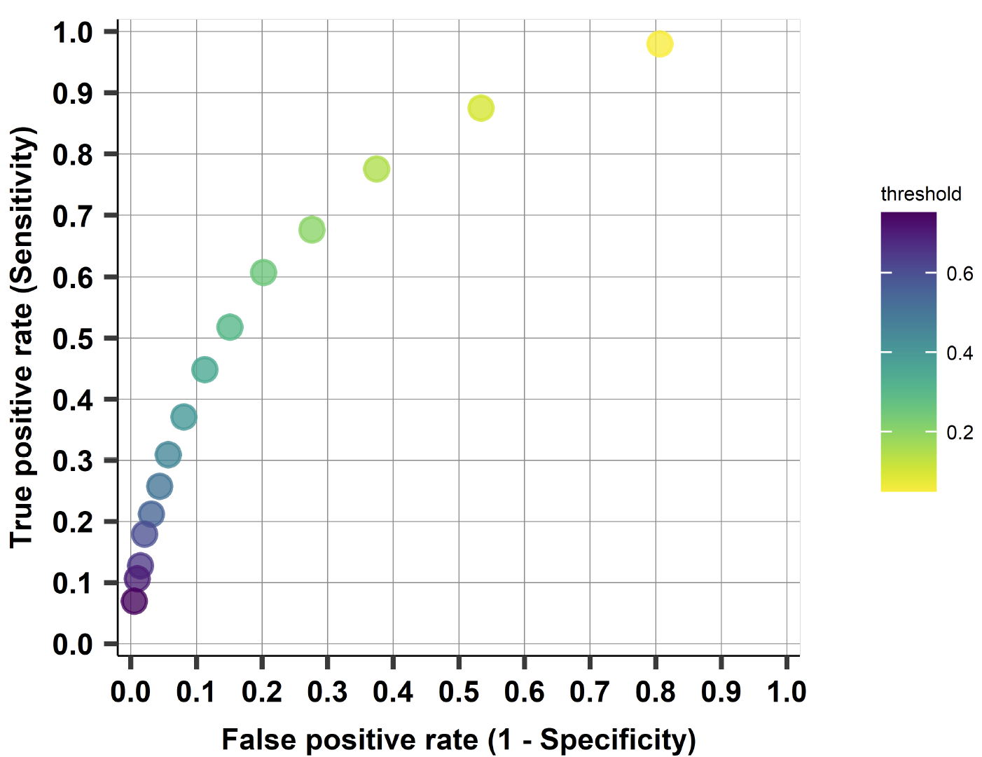
• A popular graphic for simultaneously displaying the types of errors for classification problems at various threshold values for $p^*$

• For each threshold $p^*$, we can compute confusion matrix –> calculate sensitivity and specificity

• The ROC curve of

  • a completely random probability prediction is the 45 degree line
  • a perfect probability prediction would jump from zero to one and stay at one

Visualisation of the trade-off using the ROC Curve

ROC plots sensitivity against 1-specificity: highlights the trade-off between false-positive and true-positive error rates as the classifier threshold is varied.

Source: "Machine Learning with R: Expert techniques for predictive modeling"

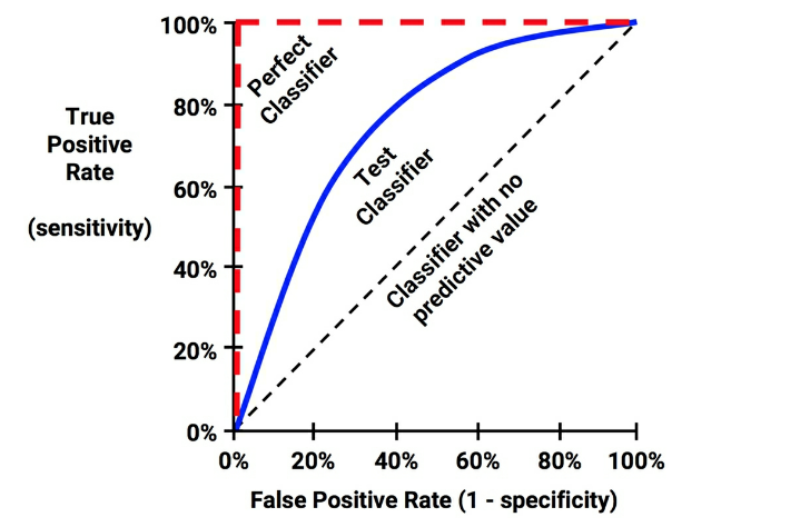
ROC Curve

• Plots true positive rate (recall) against the false positive rate ($\frac{FP}{FP + TN}$):

• For classifications from a probabilistic prediction as the threshold is moved from 0 to 1
• x-axis: False positive rate = the proportion of FP among actual negatives
• y-axis: True positive rate = the proportion of FP among actual negatives (RECALL)

ROC Curve and AUC

• The Area Under (the ROC) Curve (AUC) is a popular metric ranging between:

  • 0.5

    • random classification
    • ROC curve $=$ first diagonal

  • and 1

    • perfect classification
    • $=$ area of the square

  • better classifier $\rightarrow$ ROC curve toward the top-left corner

• Good measure for model comparison

Performance on the training set

train_accuracy = accuracy_score(y_train, y_train_hat)*100
train_auc_roc = roc_auc_score(y_train, y_train_hat_probs)*100

print('Confusion matrix:\n', confusion_matrix(y_train, y_train_hat))
print('Training AUC: %.4f %%' % train_auc_roc)
print('Training accuracy: %.4f %%' % train_accuracy)

Confusion matrix:
 [[78  8]
 [ 5 89]]
Training AUC: 98.1321 %
Training accuracy: 92.7778 %

Test set

# Predictions on the test set
y_test_hat = model1.predict(X_test)
y_test_hat_probs = model1.predict_proba(X_test)[:,1] # Probabilities of being in class 1

# Metrics
test_accuracy = accuracy_score(y_test, y_test_hat)*100
test_auc_roc = roc_auc_score(y_test, y_test_hat_probs)*100

print("Accuracy in test data {} vs. in train data {}".format(test_accuracy, train_accuracy) )
print("AUC in test data {} vs. in train data {}".format(test_auc_roc, train_auc_roc) )

Accuracy in test data 91.11111111111111 vs. in train data 92.77777777777779
AUC in test data 96.6 vs. in train data 98.13211281543789

print(classification_report(y_test, y_test_hat, digits=2))

              precision    recall  f1-score   support

           0       0.83      1.00      0.91        20
           1       1.00      0.84      0.91        25

    accuracy                           0.91        45
   macro avg       0.92      0.92      0.91        45
weighted avg       0.93      0.91      0.91        45

Plot the ROC curve

from sklearn import metrics

fpr, tpr, threshold = metrics.roc_curve(y_test, y_test_hat_probs)
print("tresholds:",  len(threshold))
roc_auc = metrics.auc(fpr, tpr)
roc_auc

tresholds: 8

0.966

import matplotlib.pyplot as plt
plt.title('Receiver Operating Characteristic')
plt.plot(fpr, tpr, 'b', label = 'AUC = %0.2f' % roc_auc)
plt.plot([0, 1], [0, 1],'r--')
plt.ylabel('True Positive Rate')
plt.xlabel('False Positive Rate')
plt.show()

We can further try to improve this model performance by hyperparameter tuning by changing the value of C or choosing other solvers available in LogisticRegression().