%%HTML
<link rel="stylesheet" type="text/css" href="https://raw.githubusercontent.com/malkaguillot/Foundations-in-Data-Science-and-Machine-Learning/refs/heads/main/docs/utils/custom.css">
%%HTML
<link rel="stylesheet" type="text/css" href="../utils/custom.css">
Foundations in Data Science and Machine Learning
Module 6: Natural Language Processing
Malka Guillot
Table of Contents
- Prologue
- Dictionary methods
- Tokenization
- Measures of document distances
- Topic models
- Embeddings
Prologue
Motivation
Much of economic research has been using structured data
Usually stored in a relational database
Sometimes called relational data
Can be easily mapped into specific fields
Research involving unstructured data is on the rise
- Text, images/videos, audio recordings, ... → treasures for (social science) researchers
- Has long required analysis by humans
- With machine learning and AI, tools to work with vast quantities of such data
[Motivation] The rise of text data
This trend is in large part due to the digitization of our societies.
The digital era generates considerable amounts of text.
- Social media and internet queries
- Wikipedia, online newspapers, TV transcripts
- Digitized books, speeches, laws
It is matched with a similar increase in computational resources.
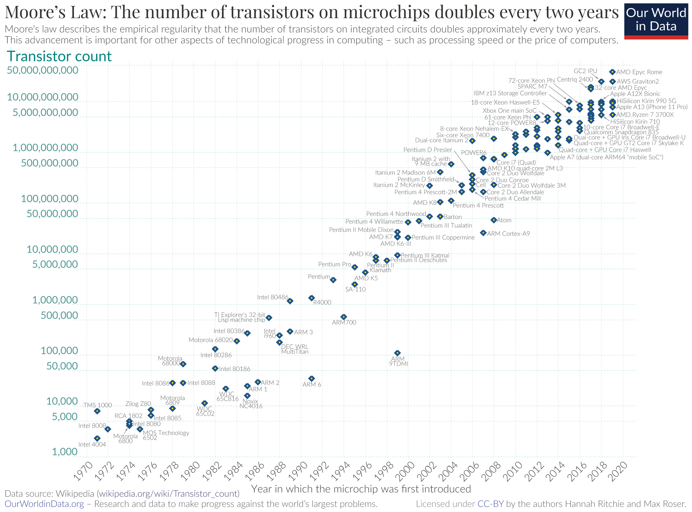
- Moore’s law = processing power of computers doubles every two years (since the 70s!)
[Motivation] Moore’s law
= Processing power of computers doubles every two years (since the 70s!)
Natural language processing
Natural language processing is a data-driven approach to the analysis of text documents.
Applications in your everyday life:
- Search engines, translation services, spam detection
Applications in social science:
- Measuring economic policy uncertainty, news sentiment, racial and misogynistic bias, political and economic narratives, speech polarization
- Predicting protests, GDP growth, financial market fluctuations
This course
Focus on natural language processing in applied economic research
Contents:
- Dictionary-based methods, measures of text distance, topic models, embeddings, supervised learning
Why is this useful for economic research?
- Measure economic/political/social concepts in texts
- New variables
- “Old” variables in new ways (e.g., more easily/flexibly)
- Use text-based variables as regressors or outcomes
- Assess the real-world impacts of language on government and the economy.
- In particular: new avenues to assess the relationship between the economy/politics and language
- Measure economic/political/social concepts in texts
A special characteristic of text data: high dimensionality
Text is very high-dimensional
Sample of documents, each $n_L$ words long, drawn from vocabulary of $n_V$ words.
The unique representation of each document has dimension $n_V^{n_L}$ .
- For example: take a sample of 30-word Twitter messages using only the one thousand most common words in the English language
- $\rightarrow$ Dimensionality $= 1000^{30} = 10^{32}$
- For example: take a sample of 30-word Twitter messages using only the one thousand most common words in the English language
“Text as Data” by Gentzkow, Kelly, Taddy (2017)
Summarize the analysis in three steps:
- Convert raw text $D$ to numerical array $\mathbf{C}$
- The elements of $\mathbf{C}$ are counts over tokens (words or phrases)
- Map $\mathbf{C}$ to predicted values $\mathbf{\hat V}$ of unknown outcomes $\mathbf{V}$
- Learn $\mathbf{\hat V(C)}$ using machine learning
- Supervised learning: for some labeled $C_i$ and $V_i$
- Unsupervised learning: topics/dimensions just from $\mathbf{C}$
- Use $\hat V$ for subsequent descriptive or causal analysis
Corpora
Plain Text
Documents
Text data is a sequence of characters called
documents The set of documents is the
corpus , which we will call $D$Text data is unstructured:
- Relevant/needed information mixed with (lots of) irrelevant unneeded information
All text data approaches throw away some information:
- Challenge: retaining valuable information
Tokenization and dimension reduction:
- Transforming an unstructured corpus $D$ to a usable matrix $X$
What counts as a document?
The unit of analysis (the “document”) varies depending on the application:
- Needs to be fine enough to fit the relevant metadata variation
- More often than not, we care about metadata!
- Should not be finer than necessary – to avoid high-dimensionality without relevant empirical variation
What should we use as the document here?
- Predicting whether a judge is right-wing or left-wing in partisan ideology, from their written opinions
- Predicting whether parliamentary speeches become more emotive in the run-up to an election
Setup the data
20 Newsgroups dataset from sklearn
We use as an example the 20 Newsgroups dataset (from sklearn), a collection of about 20,000 newsgroup (message forum) documents.
W, y = data['data'], data['target']
n_samples = y.shape[0]
n_samples
11314
y : news story categories
W : a set of documents
y[:10] # news story categories
array([ 7, 4, 4, 1, 14, 16, 13, 3, 2, 4])
One document
doc = W[0] # first document (news story)
doc[:300]
"From: lerxst@wam.umd.edu (where's my thing)\nSubject: WHAT car is this!?\nNntp-Posting-Host: rac3.wam.umd.edu\nOrganization: University of Maryland, College Park\nLines: 15\n\n I was wondering if anyone out there could enlighten me on this car I saw\nthe other day. It was a 2-door sports car, looked to be "
Store the data in a pandas dataframe
df = pd.DataFrame(W,columns=['text'])
df['topic'] = y
df.head()
| text | topic | |
|---|---|---|
| 0 | From: lerxst@wam.umd.edu (where's my thing)\nS... | 7 |
| 1 | From: guykuo@carson.u.washington.edu (Guy Kuo)... | 4 |
| 2 | From: twillis@ec.ecn.purdue.edu (Thomas E Will... | 4 |
| 3 | From: jgreen@amber (Joe Green)\nSubject: Re: W... | 1 |
| 4 | From: jcm@head-cfa.harvard.edu (Jonathan McDow... | 14 |
Dictionary methods
Dictionary methods
Dictionary-based text methods
- use a pre-selected list of words or phrases to analyze a corpus.
- Use regular expressions for this task
Corpus-specific: counting sets of words or phrases across documents
- (e.g., number of times a judge says “justice” vs. “efficiency”)
General dictionaries: WordNet, LIWC, MFD, etc
Example: dictionary methods
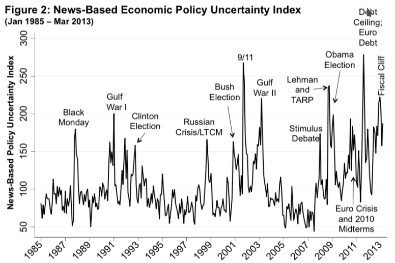
Baker, Bloom, and Davis (QJE 2016), “Measuring Policy Uncertainty”
For each newspaper on each day since 1985, tag each article mentioning:
- Uncertainty word
- Economy word
- Policy word (eg “legislation”, “regulation”)
Then, normalize the resulting article counts by the total newspaper articles that month
WordNet
- English word database: 118K nouns, 12K verbs, 22K adjectives, 5K adverbs
- Synonym sets (synsets) are a group of near-synonyms, plus a gloss (definition)
- Also contains information on antonyms (opposites), holonyms/meronyms (part-whole)
- Nouns are organized in a categorical hierarchy (hence “WordNet”)
- “hypernym” – the higher category that a word is a member of
- “hyponyms” – members of the category identified by a word
General dictionaries
Function words (e.g. for, rather, than)
- Also called stopwords (often removed)
- Can be used to get at non-topical dimensions and identify authors
LIWC (pronounced “Luke”): Linguistic Inquiry and Word Counts
- 2300 words
- 70 lists of category-relevant words, e.g. “emotion”, “cognition”, “work”, “family”, “positive”, “negative”, etc.
Mohammad and Turney (2011)
- 10,000 words coded along four emotional dimensions: joy–sadness, anger-fear, trust-disgust, anticipation-surprise
Warriner et al (2013)
- Code 14,000 words along three emotional dimensions: valence, arousal, dominance
Sentiment Analysis
- Extract a “tone” dimension – positive, negative, neutral
- Dictionaries are extensively used for sentiment analysis:
- Let $(w_i , s_i )$ be pairs of words $w_i$ and their associated sentiment score $s_i\in [−1, 1]$. e.g., (“perfect”, 0.8), (“awful”, -0.9)
- The sentiment score for any phrase $j$ of $k$ tokens is a weighted average:
$$ s_j = \frac{1}{K}\sum_{i=1}^ks_i$$
- The standard approach is lexicon-based, but they fail easily: e.g., “good” versus “not good” versus “not very good”
- The huggingface model hub has a number of transformer-based sentiment models
- Off-the-shelf scores may be trained on specific and/or biased corpora
- For example, online data
- May not work for other data, e.g., parliamentary speeches, legal texts...
Using the vaderSentimentIntensityAnalyzer from nltk
#!pip install nltk
import nltk

# Download the lexicon
nltk.download("vader_lexicon")
[nltk_data] Downloading package vader_lexicon to
[nltk_data]     /Users/malka/nltk_data...
[nltk_data]   Package vader_lexicon is already up-to-date!
True
# Import the lexicon
from nltk.sentiment.vader import SentimentIntensityAnalyzer

# Create an instance of SentimentIntensityAnalyzer
sent_analyzer = SentimentIntensityAnalyzer()

# Example
sentence = "VADER is pretty good at identifying the underlying sentiment of a text!"
print(sent_analyzer.polarity_scores(sentence))
{'neg': 0.0, 'neu': 0.585, 'pos': 0.415, 'compound': 0.75}
For the news document:
sent_analyzer = SentimentIntensityAnalyzer()
polarity = sent_analyzer.polarity_scores(doc)
print(polarity)
{'neg': 0.012, 'neu': 0.916, 'pos': 0.072, 'compound': 0.807}
Applying the sentiment analysis to the DataFrame
dfs = df.sample(frac=.2) # sample 20% of the dataset

# apply compound sentiment score to data-frame
def get_sentiment(snippet):
    return sent_analyzer.polarity_scores(snippet)['compound']

dfs['sentiment'] = dfs['text'].apply(get_sentiment)
dfs.sort_values('sentiment',inplace=True)
[x[60:150] for x  in dfs[-5:]['text']] # print beginning of most positive documents
['CLINTON: AM Press Briefing by Dee Dee Myers -- 4.15.93\nOrganization: Project GNU, Free Sof',
 ' Newsletter, Part 2/4\nReply-To: david@stat.com (David Dodell)\nDistribution: world\nOrganiza',
 "CLINTON: President's Remarks at Town Hall Meeting\nOrganization: MIT Artificial Intelligenc",
 'Final Public Dragon Magazine Update (Last chance for public bids)\nKeywords: Dragon Magazin',
 'CLINTON: Background BRiefing in Vancouver 4.4.93\nOrganization: Project GNU, Free Software ']
NLP “bias” is statistical bias
- Sentiment scores that are trained on annotated datasets also learn from the correlated non-sentiment information
- Supervised sentiment models are confounded by correlated language factors
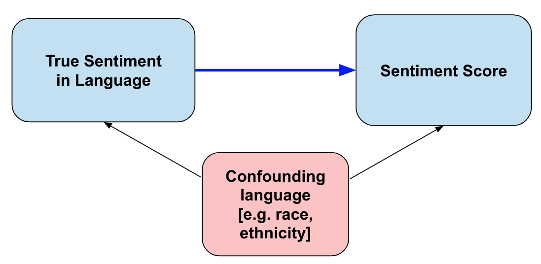
- For example, a model trained on movie reviews may learn that “good” is positive and “bad” is negative
- But it may also learn that “good” is more likely to be used in reviews of comedies, and “bad” in reviews of horror movies
(We already had this problem)
Supervised models (classifiers, regressors) learn features that are correlated with the label being annotated
Unsupervised models (topic models, word embeddings) learn correlations between topics/contexts
Dictionary methods, while having other limitations, mitigate this problem
- The researcher intentionally “regularizes” out spurious confounders with the targeted language dimension
- Helps explain why economists often still use dictionary methods...
Tokenization
Tokenization
A major goal of tokenization is to produce features that are
- Predictive in the learning task
- Interpretable by human investigators
- Tractable enough to be easy to work with
- Two broad approaches:
- Convert documents to vectors, usually frequency distributions over pre-processed $N-$ grams
- Convert documents to sequences of tokens for inputs to sequential models (e.g., BERT, GPT, etc.)
A standard tokenization pipeline
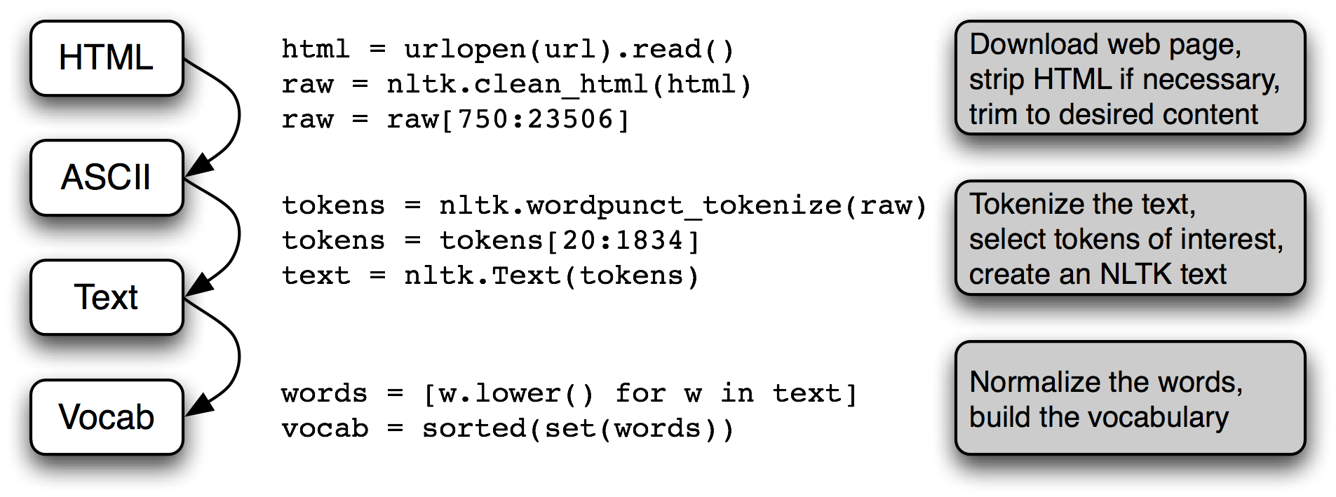
Source: 'Natural Language Processing with Python', Loper, Klein, and Bird, Chapter 3.
Example text for tokenization
text = "Marie Curie was the first woman to win a Nobel Prize, the first person to win a Nobel Prize twice, and the only person to win a Nobel Prize in 2 scientific fields. Her husband, Pierre Curie, was a co-winner of her first Nobel Prize, making them the first married couple to win the Nobel Prize and launching the Curie family legacy of 5 Nobel Prizes."
1. Pre-processing text
A key piece of the “art” of text analysis is deciding what data to throw out
- Uninformative data add noise and reduce statistical precision
- They are also computationally costly
Pre-processing choices can affect down-stream results, especially in unsupervised learning tasks (Denny and Spirling, 2018)
- Some features are more interpretable: “taxes are” / “are high” vs “taxes are high”
Capitalization
Removing capitalization is a standard corpus normalization technique
- Usually, the capitalized/non-capitalized version of a word is equivalent – e.g. words showing up capitalized at beginning of a sentence
- Capitalization uninformative
For some tasks, capitalization is important
- Required for sentence splitting, part-of-speech tagging, named entity recognition, syntactic/semantic parsing
text_lower = text.lower() # go to lower-case
text_lower
'marie curie was the first woman to win a nobel prize, the first person to win a nobel prize twice, and the only person to win a nobel prize in 2 scientific fields. her husband, pierre curie, was a co-winner of her first nobel prize, making them the first married couple to win the nobel prize and launching the curie family legacy of 5 nobel prizes.'
Remove punctuation?
Inclusion of punctuation depends on the task:
- If one vectorizes the document as a bag of words or bag of N-grams, punctuation won’t be needed
- Like capitalization, punctuation is needed for annotations (sentence splitting, parts of speech, syntax, roles, etc.) or for text generators
Drop numbers?
# recipe for fast punctuation removal
from string import punctuation
punc_remover = str.maketrans('','',punctuation)
text_nopunc = text_lower.translate(punc_remover)
print(text_nopunc)
marie curie was the first woman to win a nobel prize the first person to win a nobel prize twice and the only person to win a nobel prize in 2 scientific fields her husband pierre curie was a cowinner of her first nobel prize making them the first married couple to win the nobel prize and launching the curie family legacy of 5 nobel prizes
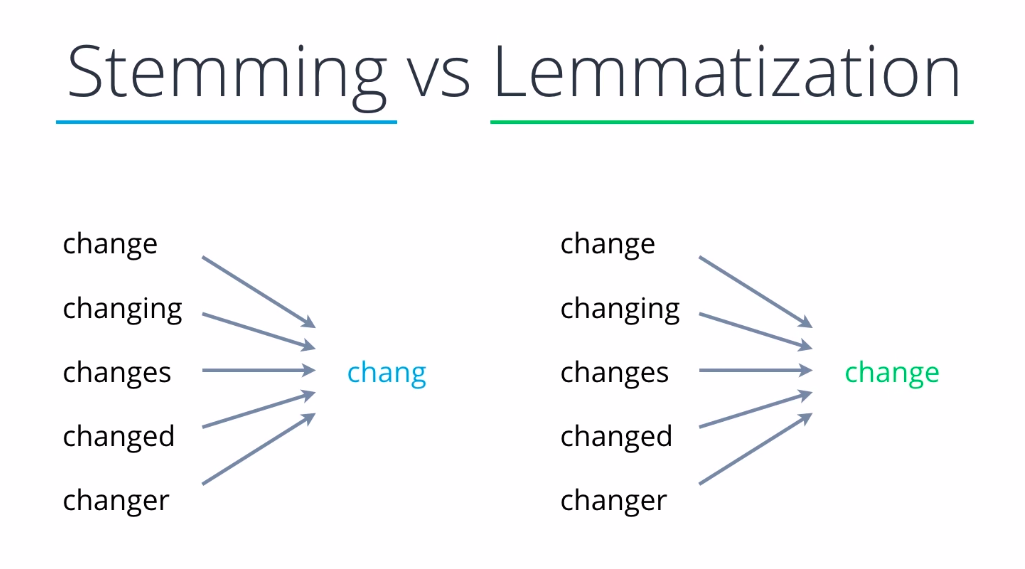
Stemming/lemmatizing
Stemming: reducing words to their root form
- e.g., “running” → “run”, “better” → “good”
- Porter stemmer, Snowball stemmer, Lancaster stemmer
Lemmatizing: reducing words to their dictionary form
- e.g., “better” → “better”, “running” → “run”
- WordNet lemmatizer, spaCy lemmatizer
from nltk.stem import SnowballStemmer
stemmer = SnowballStemmer('english') # snowball stemmer, english
# remake list of tokens, replace with stemmed versions
tokens_stemmed = [stemmer.stem(t) for t in ['tax','taxes','taxed','taxation']]
print(tokens_stemmed)
['tax', 'tax', 'tax', 'taxat']
stemmer = SnowballStemmer('german') # snowball stemmer, german
print(stemmer.stem("Autobahnen"))
autobahn
Lemmatization with WordNetLemmatizer from nltk
nltk.download('wordnet')
[nltk_data] Downloading package wordnet to /Users/malka/nltk_data...
[nltk_data]   Package wordnet is already up-to-date!
True
from nltk.stem import WordNetLemmatizer
wnl = WordNetLemmatizer()
[wnl.lemmatize(c) for c in ['corporation', 'corporations', 'corporate']]
['corporation', 'corporation', 'corporate']
Pre-processing function (homemade)
from string import punctuation
translator = str.maketrans('','',punctuation)
from nltk.corpus import stopwords
stoplist = set(stopwords.words('english'))
from nltk.stem import SnowballStemmer
stemmer = SnowballStemmer('english')

def normalize_text(doc):
    "Input doc and return clean list of tokens"
    doc = doc.replace('\r', ' ').replace('\n', ' ')
    lower = doc.lower() # all lower case
    nopunc = lower.translate(translator) # remove punctuation
    words = nopunc.split() # split into tokens
    nostop = [w for w in words if w not in stoplist] # remove stopwords
    no_numbers = [w if not w.isdigit() else '#' for w in nostop] # normalize numbers
    stemmed = [stemmer.stem(w) for w in no_numbers] # stem each word
    return stemmed
Applying the pre-processing function to the DataFrame
df['tokens_cleaned'] = df['text'].apply(normalize_text)
df['tokens_cleaned'].head(5)
0    [lerxstwamumdedu, where, thing, subject, car, ...
1    [guykuocarsonuwashingtonedu, guy, kuo, subject...
2    [twillisececnpurdueedu, thoma, e, willi, subje...
3    [jgreenamb, joe, green, subject, weitek, p9000...
4    [jcmheadcfaharvardedu, jonathan, mcdowel, subj...
Name: tokens_cleaned, dtype: object
Pre-processing function (readymade)
Shortcut: gensim.simple_preprocess.
from gensim.utils import simple_preprocess
print(simple_preprocess(text))
['marie', 'curie', 'was', 'the', 'first', 'woman', 'to', 'win', 'nobel', 'prize', 'the', 'first', 'person', 'to', 'win', 'nobel', 'prize', 'twice', 'and', 'the', 'only', 'person', 'to', 'win', 'nobel', 'prize', 'in', 'scientific', 'fields', 'her', 'husband', 'pierre', 'curie', 'was', 'co', 'winner', 'of', 'her', 'first', 'nobel', 'prize', 'making', 'them', 'the', 'first', 'married', 'couple', 'to', 'win', 'the', 'nobel', 'prize', 'and', 'launching', 'the', 'curie', 'family', 'legacy', 'of', 'nobel', 'prizes']
df['tokens_simple'] = df['text'].apply(simple_preprocess)
df['tokens_simple'].head(5)
0    [from, lerxst, wam, umd, edu, where, my, thing...
1    [from, guykuo, carson, washington, edu, guy, k...
2    [from, twillis, ec, ecn, purdue, edu, thomas, ...
3    [from, jgreen, amber, joe, green, subject, re,...
4    [from, jcm, head, cfa, harvard, edu, jonathan,...
Name: tokens_simple, dtype: object
2. Count and frequencies
Tokens
Token $=$ the most basic unit of representation in a text
A token is a sequence of characters that we want to treat as a group
- Usually, a word
- But could be a phrase, a number, a punctuation mark, etc.
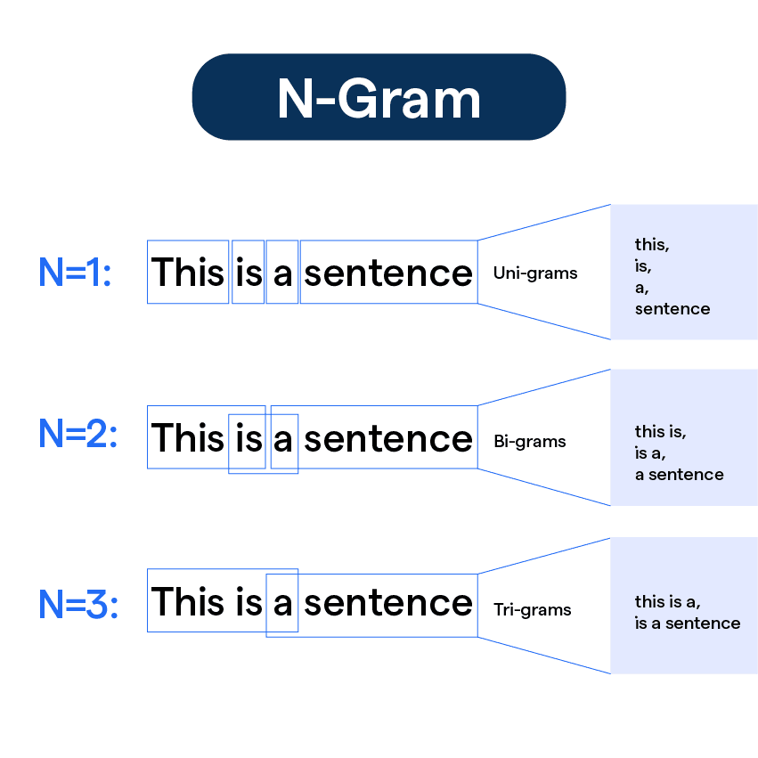
- $N-$ grams: sequences of $N$ tokens
- Moving window, for instance “hello world, i am online now” becomes “(hello world),(world i), (i am), (am online), (online now)”
- Learn a vocabulary of phrases and tokenize those: “Liège University → liege_university”
tokens = text_nopunc.split() # splits a string on white space
print(tokens)
['marie', 'curie', 'was', 'the', 'first', 'woman', 'to', 'win', 'a', 'nobel', 'prize', 'the', 'first', 'person', 'to', 'win', 'a', 'nobel', 'prize', 'twice', 'and', 'the', 'only', 'person', 'to', 'win', 'a', 'nobel', 'prize', 'in', '2', 'scientific', 'fields', 'her', 'husband', 'pierre', 'curie', 'was', 'a', 'cowinner', 'of', 'her', 'first', 'nobel', 'prize', 'making', 'them', 'the', 'first', 'married', 'couple', 'to', 'win', 'the', 'nobel', 'prize', 'and', 'launching', 'the', 'curie', 'family', 'legacy', 'of', '5', 'nobel', 'prizes']
Removing numbers
# remove numbers (keep if not a digit)
no_numbers = [t for t in tokens if not t.isdigit()]
print(no_numbers )
['marie', 'curie', 'was', 'the', 'first', 'woman', 'to', 'win', 'a', 'nobel', 'prize', 'the', 'first', 'person', 'to', 'win', 'a', 'nobel', 'prize', 'twice', 'and', 'the', 'only', 'person', 'to', 'win', 'a', 'nobel', 'prize', 'in', 'scientific', 'fields', 'her', 'husband', 'pierre', 'curie', 'was', 'a', 'cowinner', 'of', 'her', 'first', 'nobel', 'prize', 'making', 'them', 'the', 'first', 'married', 'couple', 'to', 'win', 'the', 'nobel', 'prize', 'and', 'launching', 'the', 'curie', 'family', 'legacy', 'of', 'nobel', 'prizes']
# keep if not a digit, else replace with "#"
norm_numbers = [t if not t.isdigit() else '#'
                for t in tokens ]
print(norm_numbers)
['marie', 'curie', 'was', 'the', 'first', 'woman', 'to', 'win', 'a', 'nobel', 'prize', 'the', 'first', 'person', 'to', 'win', 'a', 'nobel', 'prize', 'twice', 'and', 'the', 'only', 'person', 'to', 'win', 'a', 'nobel', 'prize', 'in', '#', 'scientific', 'fields', 'her', 'husband', 'pierre', 'curie', 'was', 'a', 'cowinner', 'of', 'her', 'first', 'nobel', 'prize', 'making', 'them', 'the', 'first', 'married', 'couple', 'to', 'win', 'the', 'nobel', 'prize', 'and', 'launching', 'the', 'curie', 'family', 'legacy', 'of', '#', 'nobel', 'prizes']
Removing stopwords
from nltk.corpus import stopwords # Stopwords
stoplist = stopwords.words('english')
# keep if not a stopword
nostop = [t for t in norm_numbers if t not in stoplist]
print(nostop)
['marie', 'curie', 'first', 'woman', 'win', 'nobel', 'prize', 'first', 'person', 'win', 'nobel', 'prize', 'twice', 'person', 'win', 'nobel', 'prize', '#', 'scientific', 'fields', 'husband', 'pierre', 'curie', 'cowinner', 'first', 'nobel', 'prize', 'making', 'first', 'married', 'couple', 'win', 'nobel', 'prize', 'launching', 'curie', 'family', 'legacy', '#', 'nobel', 'prizes']
# Counter is a quick pure-python solution.
from collections import Counter
freqs = Counter(tokens)
freqs.most_common()[:10]
[('the', 6),
 ('nobel', 6),
 ('prize', 5),
 ('first', 4),
 ('to', 4),
 ('win', 4),
 ('a', 4),
 ('curie', 3),
 ('was', 2),
 ('person', 2)]
3. N-grams
- N-grams are phrases, sequences of words up to length N.
- Bigrams, trigrams, quadgrams, etc
- Bigrams, trigrams, quadgrams, etc
N-grams and high dimensionality
- N-grams will blow up the feature space:
- Thus, filtering out uninformative N-grams is necessary
- The right number of features depends on the application
- I have gotten good performance with e.g., 2000 features
- For supervised learning tasks, a decent “rule of thumb” is to build a vocabulary of 60K, then use feature selection to get down to 10K
from nltk import ngrams
from collections import Counter

# get n-gram counts for 10 documents
grams = []
for i, row in df.iterrows():
    tokens = row['text'].lower().split() # get tokens
    for n in range(2,4):
        grams += list(ngrams(tokens,n)) # get bigrams, trigrams, and quadgrams
    if i > 50:
        break
Counter(grams).most_common()[:8]  # most frequent n-grams
[(('of', 'the'), 41),
 (('subject:', 're:'), 37),
 (('in', 'the'), 33),
 (('to', 'the'), 27),
 (('i', 'am'), 21),
 (('i', 'have'), 21),
 (('to', 'be'), 19),
 (('on', 'the'), 18)]
4. Parts of speech
Parts of speech (POS) tags provide useful word categories corresponding to their functions in sentences
- Eight main parts of speech: verb (VB), noun (NN), pronoun (PR), adjective (JJ), adverb (RB), determinant (DT), preposition (IN), conjunction (CC).
POS vary in their informativeness for various functions
- For categorizing topics, nouns are usually most important
- For sentiment, adjectives are usually most important
One can count POS tags as features – e.g., using more adjectives, or using more passive verbs
POS n-gam frequencies (e.g. NN, NV, VN, ...), like function words, are good stylistic features for authorship detection
- Not biased by topics/content
Install spaCy and download the model
pip install spacy
python -m spacy download en_core_web_sm
import spacy
nlp = spacy.load('en_core_web_sm')
Parts of speech tagging with spaCy
dfs = df.sample(10)
dfs['doc'] = dfs['text'].apply(nlp)
doc = dfs['doc'].iloc[0]

for token in doc[:10]:
    print(f"Token: {token.text}, POS: {token.pos_}")
Token: From, POS: ADP
Token: :, POS: PUNCT
Token: wcd82671@uxa.cso.uiuc.edu, POS: PROPN
Token: (, POS: PUNCT
Token: daniel, POS: PROPN
Token: warren, POS: PROPN
Token: c, POS: PROPN
Token: ), POS: PUNCT
Token:
, POS: SPACE
Token: Subject, POS: NOUN
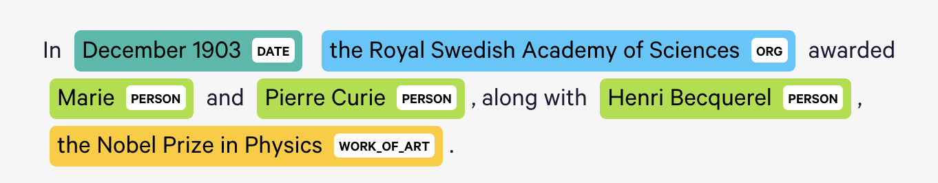
5. Named Entity Recognition
Refers to the task of identifying named entities such as "December 1903" and Pierre Curie”, which can be used as tokens
Detecting the type requires a trained model (e.g. spaCy)
- Common types: persons, organizations, locations, dates, etc.
# spacy NER noun chunks
chunks = list(nlp(df['text'].iloc[10]).noun_chunks)
chunks[:20]
[irwin@cmptrc.lonestar.org,
 (Irwin Arnstein,
 Subject,
 Recommendation,
 Duc
 Summary,
 What,
 it,
 Distribution,
 usa,
 Sat,
 May 1993 05:00:00 GMT
 Organization,
 CompuTrac Inc.,
 Richardson TX
 Keywords,
 Ducati,
 GTS,
 I,
 a line,
 a Ducati 900GTS 1978 model,
 the clock,
 paint]
Bag-of-words representation
The most common way to represent text data $D$ (ie a corpus) is as a matrix $X$ of token counts
- Each row is a document, each column is a token
- The value in each cell is the count of that token in that document
More generally, “bag-of-terms” representation refers to counts over any informative features – e.g. N-grams, syntax features, etc.
scikit-learn's CountVectorizer
from sklearn.feature_extraction.text import CountVectorizer
vec = CountVectorizer(min_df=0.001, # at min 0.1% of docs
                        max_df=.8, # drop if shows up ih more than 80%
                        max_features=1000,
                        stop_words='english',
                        ngram_range=(1,3)) # words, bigrams, and trigrams
X = vec.fit_transform(df['text'])

# save the vectors
# pd.to_pickle(X,'X.pkl')

# save the vectorizer
# (so you can transform other documents, also for the vocab)
#pd.to_pickle(vec, 'vec-3grams-1.pkl')

X
<11314x1000 sparse matrix of type '<class 'numpy.int64'>'
	with 526707 stored elements in Compressed Sparse Row format>
Counts and frequencies
- Document counts: number of documents where a token appears
- Term counts: number of total appearances of a token in corpus
- Term frequency: $$\text{Term Frequency of w in document d} = \frac{\text{Count of w in document d}}{\text{Total tokens in document d}}$$
Building a vocabulary
- An important featurization step is to build a vocabulary of words:
- Compute (document) frequencies for all words
- Inspect low-frequency words and determine a minimum document threshold
- For instance: 10 documents, or .25% of documents
- Can also impose more complex thresholds, e.g.:
- Appears twice in at least 20 documents
- Appears in at least 3 documents in at least 5 years
- Assign numerical identifiers to tokens to increase speed and reduce disk usage
TF-IDF (Term Frequency-Inverse Document Frequency) weighting
TF/IDF: “term-frequency / inverse-document-frequency”
The formula for word $w$ in document $k$: $$\text{TF-IDF}(w, k) = \frac{\text{Count of w in k}}{\text{Total word of k}} \times \log\left(\frac{number of documents in D}{\text{number of documents where w appears}}\right)$$
The formula up-weights relatively rare words that do not appear in all documents
- These words are probably more distinctive of topics or differences between documents
scikit-learn’s TfidfVectorizer
# tf-idf vectorizer up-weights rare/distinctive words
from sklearn.feature_extraction.text import TfidfVectorizer
tfidf = TfidfVectorizer(min_df=0.001,
                        max_df=0.9,
                        max_features=1000,
                        stop_words='english',
                        use_idf=True, # the new piece
                        ngram_range=(1,2))

X_tfidf = tfidf.fit_transform(df['text'])
#pd.to_pickle(X_tfidf,'X_tfidf.pkl')
X_tfidf
<11314x1000 sparse matrix of type '<class 'numpy.float64'>'
	with 521387 stored elements in Compressed Sparse Row format>
Measures of document distances
In economics, we often want to compare documents (broadly defined) to one another
- For instance, how close is a political speech to the party leader?
Now, we focus on methods designed to measure document distance/proximity
Almost all content from this lecture can be framed as measuring document distance in some way
- all "text representations" can be used to measure document distance
Document-term matrix
The document-term matrix $\mathbf{X}$ is a matrix where
- Each row $d$ corresponds to a document
- Each column corresponds to a term (word or token).
A matrix entry $\mathbf{X}_{[d,w]}$ quantifies the strength of association between a document $d$ and a word $w$,
- generally its count or frequency
| Document | Word1 | Word2 | Word3 | Word4 |
|---|---|---|---|---|
| Doc1 | 2 | 1 | 0 | 1 |
| Doc2 | 0 | 3 | 1 | 0 |
| Doc3 | 1 | 0 | 4 | 2 |
Each row $\mathbf{X}_{[d,:]}$ is a document vector of the distribution over terms
- These vectors have a spatial interpretation
- $\rightarrow$ geometric distances between document vectors reflect semantic distances between documents in terms of shared terms
- These vectors have a spatial interpretation
Each column $\mathbf{X}_{[:,w]}$ is term vector of a distribution over documents
- also have a spatial interpretation
- $\rightarrow$ geometric distances between term vectors reflect semantic distances between words in terms of showing up in the same documents
- also have a spatial interpretation
Cosine similarity
Each document is
- a vector $\mathbf{x}_{d}$ e.g. token counts or TF-IDF frequencies
- Similar documents have similar vectors
Can measure similarity between documents $i$ and $j$ by the cosine of the angle between $\mathbf{x_i}$ and $\mathbf{x_j}$
- With perfectly collinear documents (that is, $\mathbf{x_i} = \alpha \mathbf{x_j}$ , $\alpha > 0$), $\cos(0) = 1$
- For orthogonal documents (no words in common), $\cos(\pi/2) = 0$
Cosine similarity is computable as the normalized dot product of the two vectors: $$\text{cosine similarity}(\mathbf{x_i}, \mathbf{x_j}) = \frac{\mathbf{x_i} \cdot \mathbf{x_j}}{||\mathbf{x_i}|| \cdot ||\mathbf{x_j}||}$$
# compute pair-wise similarities between all documents in corpus"
from sklearn.metrics.pairwise import cosine_similarity

sim = cosine_similarity(X[:100])
sim.shape
(100, 100)
sim[:4,:4]
array([[1.        , 0.20384233, 0.15095711, 0.19219753],
       [0.20384233, 1.        , 0.12569587, 0.1608558 ],
       [0.15095711, 0.12569587, 1.        , 0.16531366],
       [0.19219753, 0.1608558 , 0.16531366, 1.        ]])
# TF-IDF Similarity
tsim = cosine_similarity(X_tfidf[:100])
tsim[:4,:4]
array([[1.        , 0.05129256, 0.08901433, 0.06064389],
       [0.05129256, 1.        , 0.07497709, 0.03570566],
       [0.08901433, 0.07497709, 1.        , 0.09077347],
       [0.06064389, 0.03570566, 0.09077347, 1.        ]])
Clustering
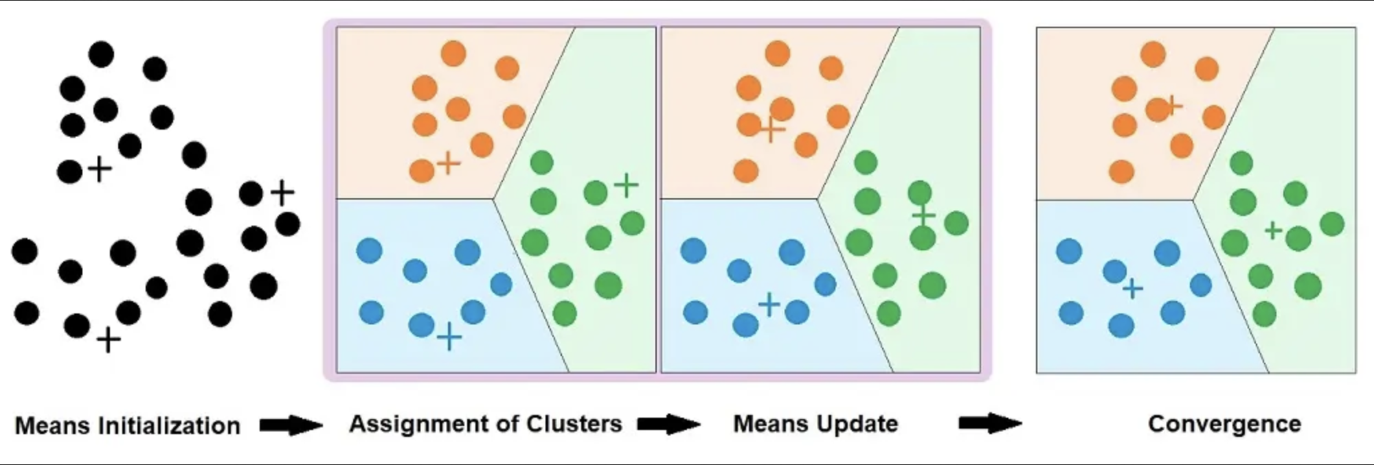
k-means clustering
Method to partition the observations (documents) into $k$ clusters $ S_1, S_2, \ldots, S_k $:
- Each cluster is represented by its centroid $ \mu_i $
- Each document is assigned to the cluster with the closest centroid
- $k$ (number of clusters) is the only hyperparameter
Algorithm:
Initialize cluster centroids randomly
Shift them around to minimize the sum of the within-cluster squared distance (features should be standardized)
$$\arg\min_{S_1, ..., S_k}\sum_{i=1}^k\sum_{x \in S_i}||x - \mu_i||^2$$
Repeat until convergence
Other clustering algorithms
“k-medoid” clustering use L1 distance rather than Euclidean distance
- Produces each cluster’s “medoid” (median vector) instead of “centroid” (mean vector)
- Less sensitive to outliers
- The medoid can be used as a representative data point
DBSCAN defines clusters as continuous regions of high density
- Detects and excludes outliers automatically
Agglomerative (hierarchical) clustering makes nested clusters
Final Notes on $\mathbf{X}$
Each row $\mathbf{X}_{[d,:]}$ is a document vector of the distribution over terms
Each column $\mathbf{X}_{[:,w]}$ is term vector of a distribution over documents
The same methods we used on the rows can be used on the columns:
- Apply cosine similarity to the columns to compare words (rather than compare documents)
- Apply $k-$means clustering to the columns to get clusters of similar words (rather than clusters of documents)
Topic models
Topic models
Summarize unstructured text
Use words within the document to infer the subject
Interpretable
A stylized example
A corpus of documents
- Doc 1: guns zombies biohazard win lose...
- Doc 2: player lose score survival...
- Doc 3: zombies survival congress...
- Doc 4: ...
- Doc 100000: congress welfare constitution guns...
What are the topics in these documents?
Zombies: guns, zombies, biohazard, survival
Sports: player, win, score, lose
Politics: welfare, congress, constitution, guns
How does it work?
Topic models
Topics models infer latent topics in the corpus:
- Documents as distributions over topics
- Topics as distributions over words
Main assumption: The number of topics $K$ is a hyperparameter.
In the original models, formally, $\mathbf{W}$ is decomposed into two matrices: $$\mathbf{W} = \mathbf{\Theta}\times \mathbf{B}^T$$ where $\mathbf{W}\in D\times V$ is the document-term matrix, $\mathbf{\Theta}\in D\times K$ is the document-topic matrix, and $\mathbf{B}\in V\times K$ is the topic-term matrix
Latent Dirichlet Allocation (LDA)
The most popular topic model
Each document is a mixture of topics
Each topic is a mixture of words
The model is generative:
- For each document, draw a distribution over topics
- For each word in the document, draw a topic from the distribution over topics
- For each word, draw a word from the distribution over words for the topic
Using an LDA model
Once trained, one can easily get topic proportions for a corpus
For any document – doesn’t have to be in training corpus
The main topic is the highest-probability topic
Documents with the highest share in a topic work as representative documents for the topic
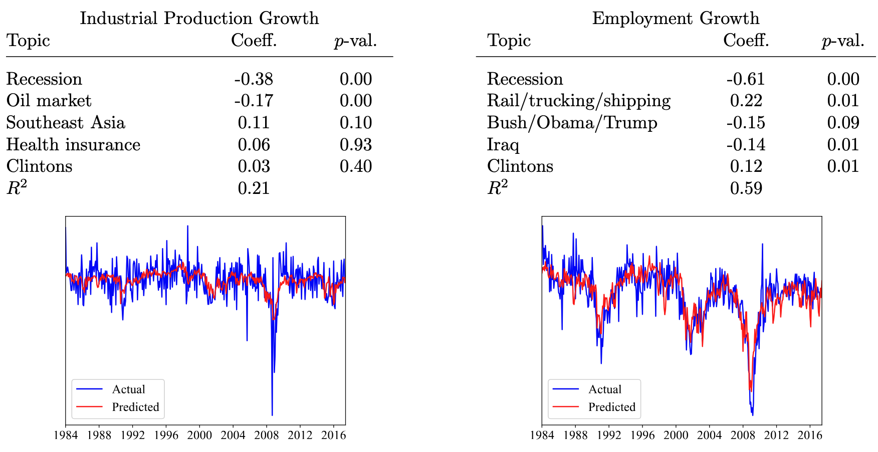
One can use the topic proportions as variables in a social science analysis
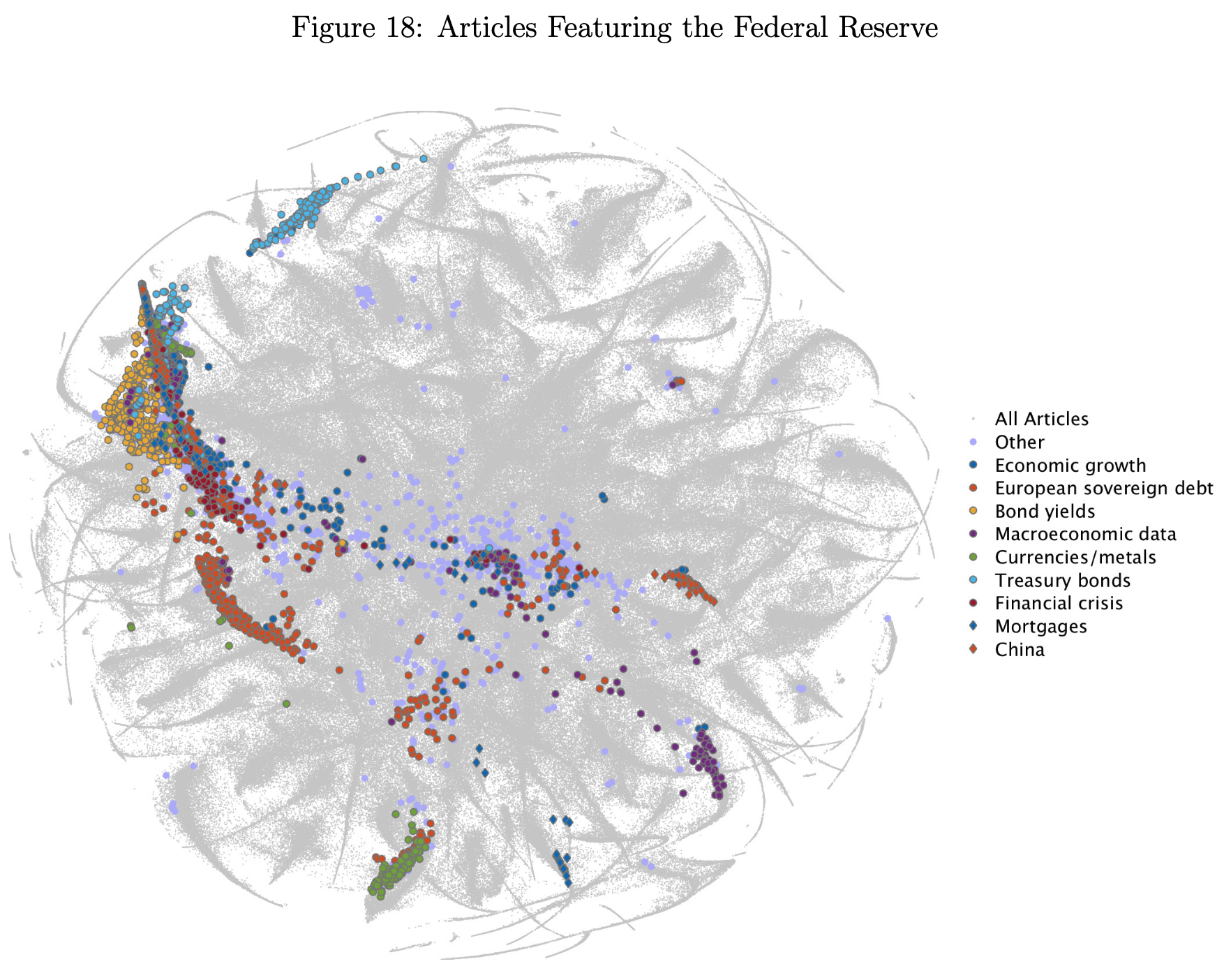
... to predict macroeconomic variables.
Word embeddings
Text classifiers
- produce $\hat y_i=f(\mathbf{x_i}, \hat\theta)$ a vector of predicted probabilities across classes for each document $i$
- $y_i$ is a vector of class probabilities ie. a compressed representation of the text features $\mathbf{x_i}$
- $\mathbf{x_i}$: matrix of features is itslef a compressed representation of the document
- the learned parameters $\hat\theta$ can be understood as a compressed representation of the data
- $\hat \theta$ contains information about the training corpus, the text features, and the oucomes.
Limitations of bag-of-words representations
Until now, $\mathbf{x_i}$ has been a “bag-of-words” representation.
Bag-of-words representations disregard syntax
- “The cat ate the mousse.” versus The mousse ate the cat.”
- $\rightarrow$ These two sentences have the same bag-of-words representation
Bag-of-words representations disregard semantic proximity between words
- “hi” and “hello” are completely distinct features for predicting whether a message is greeting somebody
- “economics” and “sociology” are distinct features for predicting whether a message is about the social sciences
Can we estimate text features that capture semantic proximity?
Word embeddings
- Fancy word, old concept
- Vector representation of a word (we have already seen count-vectorizer, tf-idf)
- What we mean by word embedding is that we are embedding a categorical entity into a vector space

Language in context (and vice-versa)
Neighboring words provide us with additional information to interpret a word’s meaning
In other words, word co-occurrences capture context
This information is useful for machine learning applications
- For example, document classification, machine translation, syntax prediction, machine comprehension, etc.
Best known word embeddings model: Word2Vec
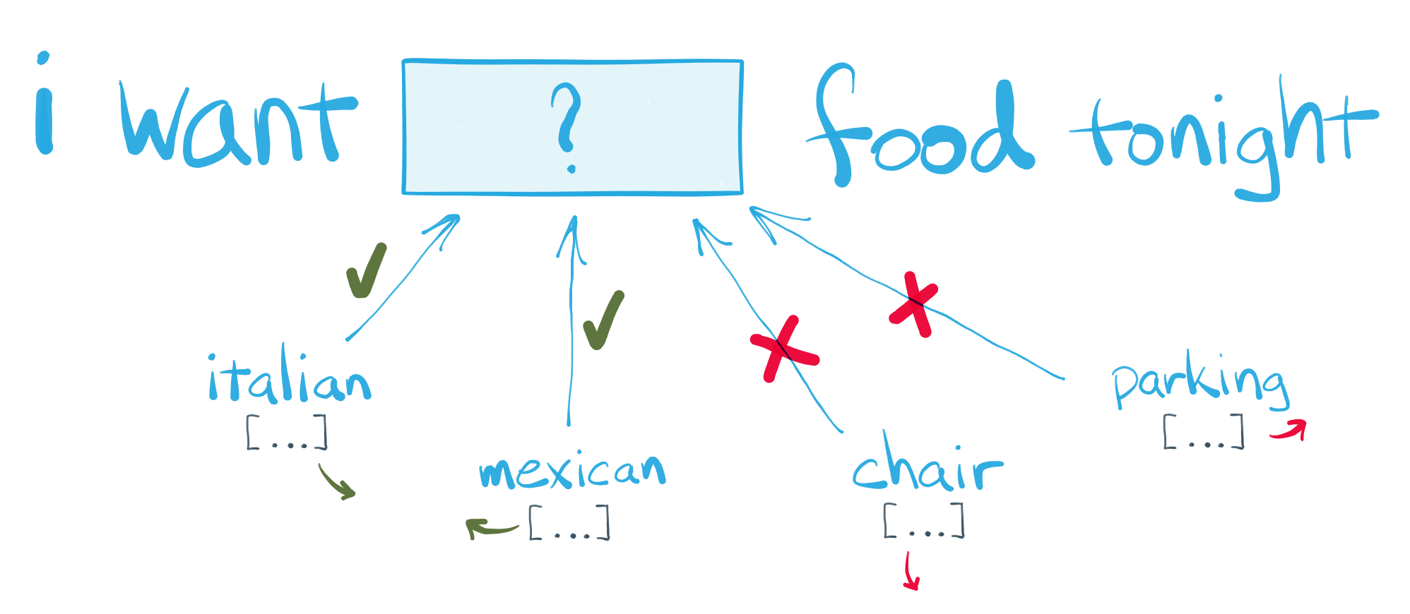
Word2Vec reformulates learning word co-occurrences as two prediction tasks:
- Continuous Bag of Words (CBOW): Given its context words, predict a focus word
- Skipgram: Given a focus word, predict all its context words
In both cases, the model results in a low-dimensional, dense vector space representation of $C$
Distance between texts
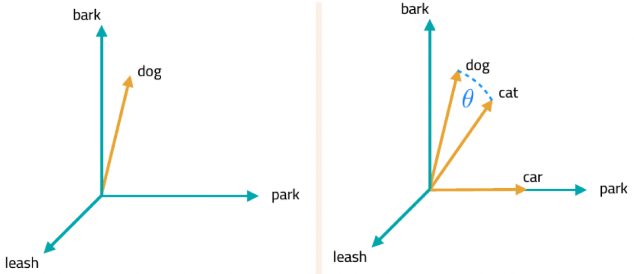
- With embeddings, we can use linear algebra to understand relationships between words
- In particular, words that are geometrically close to each other are similar
- The standard metric for comparing vectors is cosine similarity
$$\text{cosine similarity}(x_i, x_j) = \frac{x_i \cdot x_j}{||x_i|| \cdot ||x_j||}$$
- When vectors are normalized, cosine similarity is:
- Simply the dot product of both vectors
- Proportional to the Euclidean distance (so you can use it, too)
Distance between texts
Visualizing embeddings
One can also visualize the resulting embedding space by projecting it on a two-dimensional space
Three commonly used techniques are:
- Principal Component Analysis (PCA)
- t-distributed stochastic neighbor embedding (t-SNE)
- Uniform Manifold Approximation and Projection (UMAP)
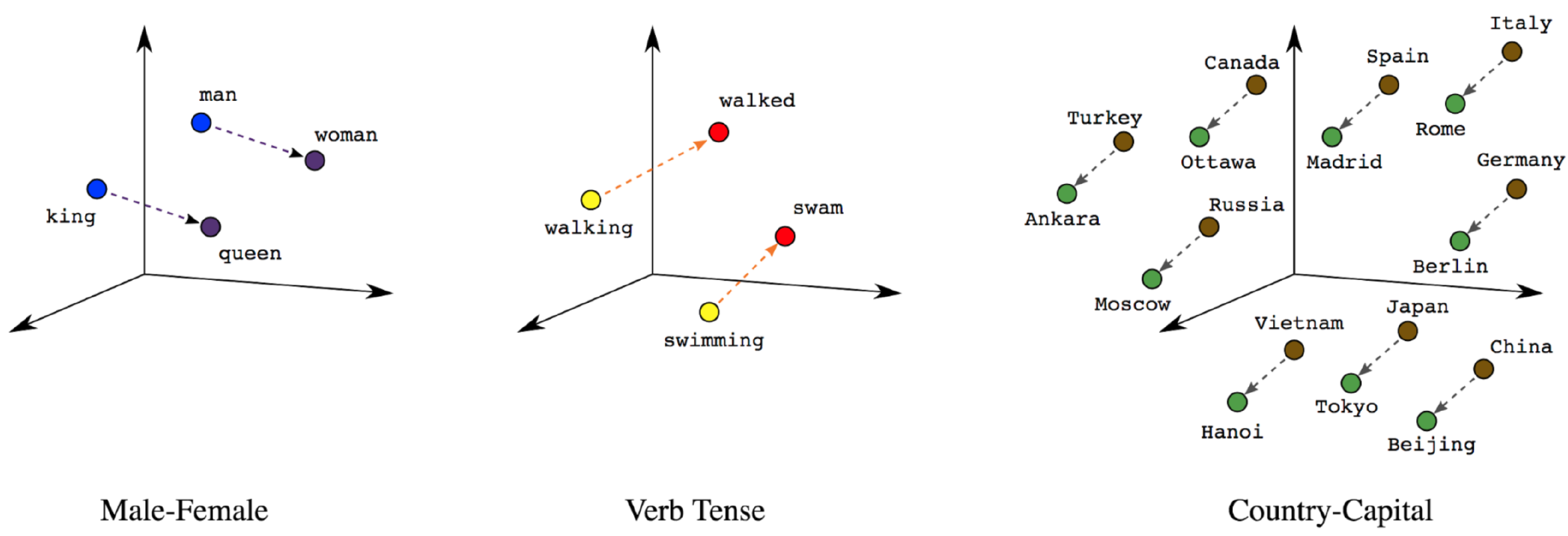
Basic arithmetic often carries meaning
Word2vec algebra can depict conceptual, analogical relationships between words.
- eg. $\overrightarrow{\text{king}} - \overrightarrow{ \text{man}} + \overrightarrow{wo⃗man} ≈ \overrightarrow{qu⃗een}$
Some refinements
The main assumption behind word2vec is that context words are exchangeable
In other words, the ordering of words is not accounted for
Recent models relax this assumption; they are called transformers...
.. and consistently outperform previous language models in various tasks
Pros and cons of embeddings
Pros:
- Many pre-trained models for different languages are freely available online
- Many packages to train models from scratch or fine-tune existing models to a specific corpus
- Often, they provide sizable gains in prediction accuracy
Cons:
- Clear loss of interpretability relative to bag-of-words
- Neighbouring words are not the only forms of context
- Often critiqued as “stochastic parrots” (Bender et al., 2021)